E Using R
E.2 How to do it in R
E.2.1 Reading data
E.2.1.1 Reading data stored in csv files
In order to read csv files with R code we can use read.csv (or read.csv2, if the csv file follows Polish regional settings, with semicolons as data separators and commas as decimal symbols).
Example E.1 Following file contains data on height of three people. Import the data to R and and calculate average height.
E.2.1.2 Reading data from Google sheets
To use the data from Google sheets one can use googlesheets4 package. The read_sheet function enables importing data to R. To avoid logging in to Google account one can use gs4_deauth.
Example E.2 Simple regression template in Google sheets can be found under the following link: https://docs.google.com/spreadsheets/d/1SwtgiYm3ljtOWsQ-wVbOQ06KLp69WpTAe35IYAkhjAg. Import the data to R and compute the standard deviation of variable Y.
E.2.2 Probability distributions
E.2.2.1 Normal distribution
Many common probability distributions are available in R in the form of four functions, which can be represented by the normal distribution as an example (see figure (fig:normilustr)):
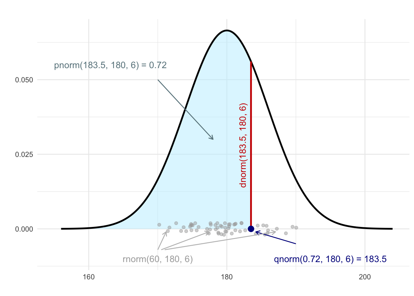
Figure E.1: Illustration of the use of the functions pnorm, qnorm, dnorm and rnorm for a normal distribution with mean equal to 180 and standard deviation equal to 6.
dnorm(x, mean = mu, sd = sigma)is the density function (9.1) of a normal distribution with meanmuand standard deviationsigma,pnorm(x, mu, sigma)is the cumulative distribution function (CDF, 7.4) of this normal distribution,qnorm(a, mu, sigma)is the quantile function of the CDF it is used, inter alia, to find the critical values (boundaries of the rejection area),rnorm(k, mu sigma)is a function that enables drawingkvalues from this normal distribution.
Example E.3 Random variable \(X\) has a normal distribution with a mean of 180 and a standard deviation of 6. Using the appropriate CDF function in R, compute \(mathbb{P}(178 < X < 183)\).
E.2.2.2 Binomial distribution
Similarly, for discrete distributions using the binomial distribution as an example:
dbinom(x, size = n, prob = p)is a probability mass function (7.1) of the binomial distribution with parametersnandp,pbinom(x, n, p)is its CDF,qbinom(a, n, p)is its quantile function,and
rbinom(k, n, p)enables random value generation from this distribution.
Example E.4 Using R, calculate the probability that tossing a symmetrical coin 20 times will return 15 or more heads.
E.2.3 Simulating using R
Useful R functions for simulation:
generating random values from distributions:
rnorm(normal distribution),runif(uniform distribution) itp.sample,replicate.
Functions such as rnorm, runif and similar functions are used to generate random variables from specific distributions. For example, rnorm(100, 4, 2) will generate 100 values from a normal distribution with mean 4 and standard deviation 2.
The sample function allows you to randomly select values from a given set, shuffle (permutate) a set or draw samples with specific probabilities. For example:
sample(1:200, 5)draws five integers from the set from 1 to 200,sample(0:9)represents a random permutation (reshuffling) of single-digit numbers,the
replace=TRUEoption allows a draw with repetitions, hence 10 results of a dice throw can be generated by writingsample(1:6, 10, replace=TRUE),the
prob=option allows us to set the probabilities, hence the codesample(c('H', ‘T’), size=20, prob=c(0.6, 0.4), replace=TRUE)generates 20 results of a non-symmetric coin toss where the probability of heads (H) is 0.6.
The replicate function allows you to generate (and store) the results of repeating some calculation containing a random element. For example, using the code results <- replicate(1000, mean(rnorm(100, 180, 6)))), it is possible to store in the results vector 1000 averages from 100-element samples derived from a normal distribution with mean 180 and standard deviation 6.