5 Bayes’ formula
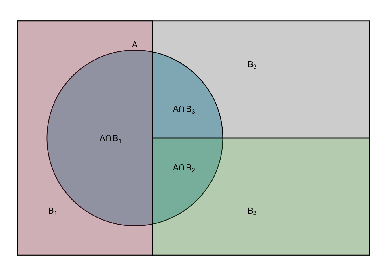
A partition of the sample space \(\Omega\) is a set of mutually exclusive (\(B_i \cap B_j = \emptyset\)) events \(B_1, B_2, ..., B_k\) whose sum constitutes the entire space (\(\Omega = B_1 \cup B_2 \cup ... \cup B_k\)).
5.1 Law of total probability
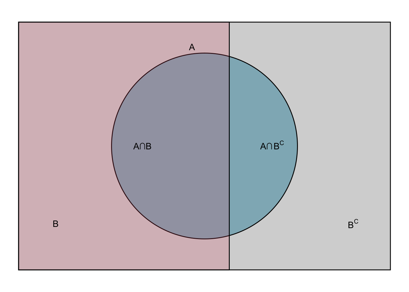
Binary partition (\(B\) and \(B^C\)):
\[\begin{equation} \mathbb{P}(A) = \mathbb{P}(A \cap B) + \mathbb{P}(A \cap B^c) \tag{5.1} \end{equation}\]
\[\begin{equation} \mathbb{P}(A) = \mathbb{P}(A|B)\mathbb{P}(B) + \mathbb{P}(A|B^c)\mathbb{P}(B^c) \tag{5.2} \end{equation}\]
Multi-part partition:
\[\begin{equation} \mathbb{P}(A)=\sum_i \mathbb{P}(A \cap B_i) \tag{5.3} \end{equation}\]
\[\begin{equation} \mathbb{P}(A)=\sum_i \mathbb{P}(A|B_i)\mathbb{P}(B_i) \tag{5.4} \end{equation}\]
5.2 Bayes’ theorem
For a binary partition (\(H\) – the hypothesis is true vs \(H^c\) – the hypothesis is not true):
\[\begin{equation} \mathbb{P}(H|D) = \frac{\mathbb{P}(D|H)\times \mathbb{P}(H)}{\mathbb{P}(D)} = \frac{\mathbb{P}(D|H)\times \mathbb{P}(H)}{\mathbb{P}(D|H)\mathbb{P}(H) + \mathbb{P}(D|H^c)\mathbb{P}(H^c)} \tag{5.5} \end{equation}\]
Similarly, in the case of a multi-part partition (\({H_i}\) are competing disjoint hypotheses exhausting all possibilities):
\[\begin{equation} \mathbb{P}(H|D) = \frac{\mathbb{P}(D|H)\times \mathbb{P}(H)}{\mathbb{P}(D)} = \frac{\mathbb{P}(D|H)\times \mathbb{P}(H)}{\sum_i{\mathbb{P}(D|H_i)\mathbb{P}(H_i)}} \tag{5.6} \end{equation}\]
In the formula, instead of the cliched \(A\) and \(B\) the notations \(H\) for a “hypothesis” and \(D\) for „data”, are used to illustrate how Bayes’ theorem can be (and is) used.
Before we get new data, we assume that the probability of our hypothesis is \(\mathbb{P}(H)\). This probability \(\mathbb{P}(H)\) is called the prior probability).
Once we have new data (\(D\)), we get a changed probability of the hypothesis \(\mathbb{P}(H|D)\), the posterior probability.
To calculate posterior probabilities given the new data \(D\), we utilize the likelihood \(\mathbb{P}(D|H)\), the probability of data given the hypothesis.
In the Bayes’ formula we also use the total probability of the data \(\mathbb{P}(D)\) determined most often using the law of total probability (the formulas (5.1) – (5.4)).
Bayes’ theorem can be remembered as follows: the posterior is proportional to the product of the prior and the likelihood. Symbolically:
\[Posterior \propto Prior \times Likelihood\]
5.3 Examples
Example 5.1 Suppose we are dealing with a relatively rare disease. In the population, one in 1,000 people have it. We also have an imperfect test that is supposed to detect the disease. Its sensitivity (the probability that it will return a positive result—that is, detect the disease—in a person who has the disease) is 0.95. The probability of a false positive result in a healthy person is 0.01.
We randomly select a person from the population and apply the test in question. It returns a positive result. What is the probability that this person has the disease?
We have two hypotheses (a binary partition): \(H\) – the randomly selected person has the disease and \(H^C\) – the person is not sick. The prior probabilities are \(\mathbb{P}(H) = 0.001\) and \(\mathbb{P}(H^C) = 0.999\). Our data \(D\) here is the positive result of the test. Likelihood probabilities, i.e. the probabilities of obtaining positive test given the hypothesis \(H\) or \(H^C\) is true, are \(\mathbb{P}(D|H)=0.95\) and \(\mathbb{P}(D|H^C) = 0.01\), respectively. We are looking for the probability the person is sick given we already know the data (the positive result of the test): \(\mathbb{P}(H|D)\).
Using the Bayes’ formula:
\(\mathbb{P}(H|D) = \frac{\mathbb{P}(D|H)\times \mathbb{P}(H)}{\sum_i{\mathbb{P}(D|H_i)\mathbb{P}(H_i)}} = \frac{0.95\times 0.001}{0.95\times 0.001+0.01\times 0.999} \approx 0.0868\)
The posterior probability that the randomly selected person has the disease is about 8.68%.
5.4 Templates
R code
# Hypotheses: descriptions (optional)
hypotheses <- c("Disease", "No disease")

# Prior
prior <- c(.001, .999)

# Likelihood
likelihood <- c(.95, .01)

# Posterior
posterior <- prior*likelihood
posterior <- posterior/sum(posterior)

# Check
if(length(prior)!=length(likelihood))
{print("Both vectors (prior and likelihood) should be the same length. ")}
if(sum(prior)!=1){
  print("Suma prawdopodobieństw w rozkładzie zaczątkowym (prior) powinna być równa 1.")}
if (!exists("hypotheses") || length(hypotheses)!=length(prior)) {
  hipotezy <- paste0('H', 1:length(prior))
}

# Wynik w formie ramki danych:
print(data.frame(
  Hypothesis = hypotheses, `Prior` = prior, `Likelihood` = likelihood, `Posterior` = posterior
))
## Hypothesis Prior Likelihood Posterior
## 1 Disease 0.001 0.95 0.08683729
## 2 No disease 0.999 0.01 0.91316271# Chart
library(ggplot2)
hypotheses<-factor(hypotheses, levels=hypotheses)
df <- data.frame(Hypotheses = c(hypotheses, hypotheses),
`Distribution` = factor(c(rep("prior", length(prior)), rep("posterior", length(posterior))),
levels=c("prior", "posterior")
),
`Probability` = c(prior, posterior)
)
ggplot(data=df, aes(x=Hypotheses, y=`Probability`, fill=`Distribution`)) +
geom_bar(stat="identity", position=position_dodge())+
geom_text(aes(label = format(round(`Probability`,4), nsmall=4), group=`Distribution`),
position = position_dodge(width = .9), vjust = -0.2)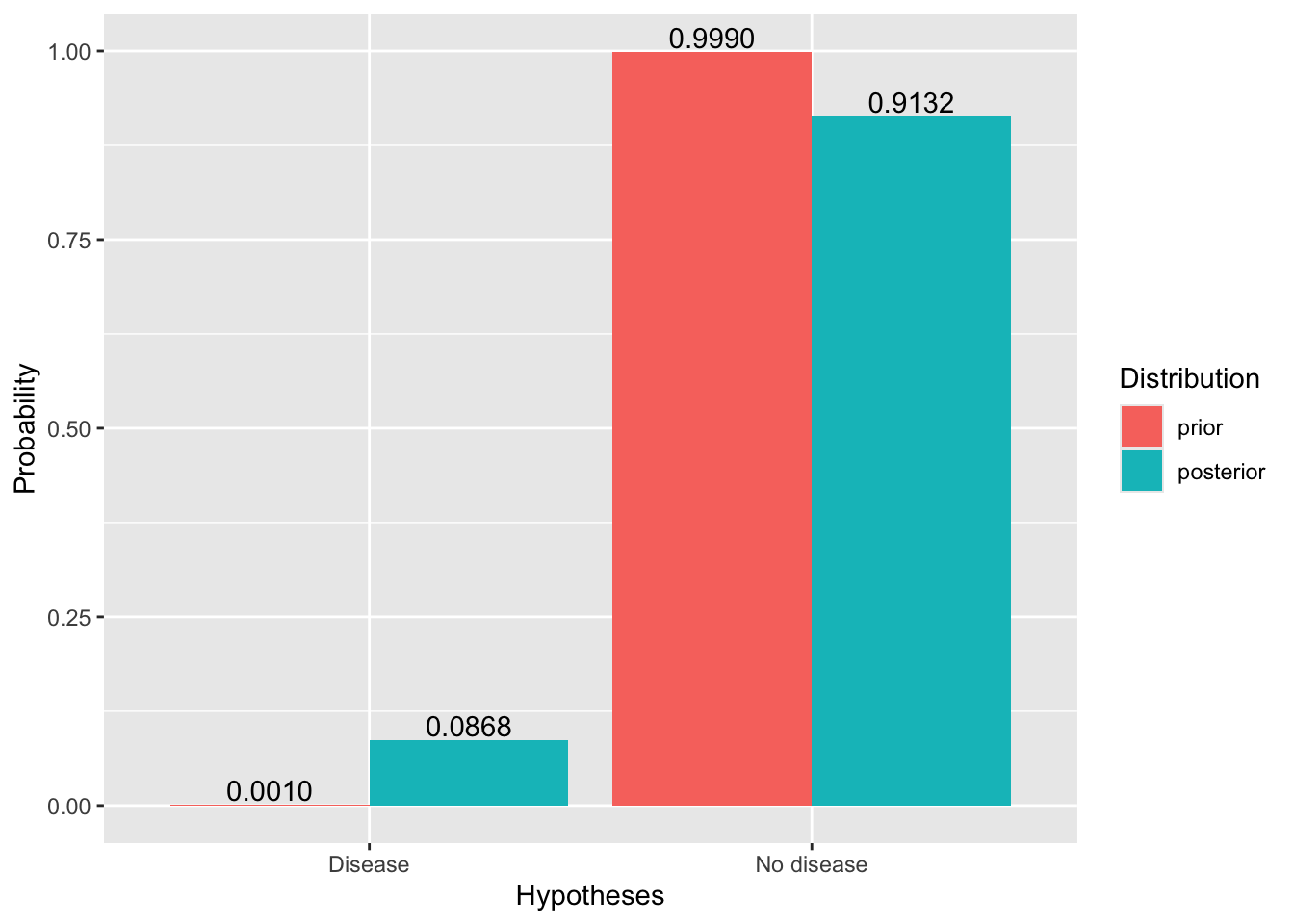
Python code
# Hypotheses: descriptions (optional)
hypotheses = ["Disease", "No disease"]

# Prior
prior = [.001, .999]

# Likelihood
likelihood = [.95, .01]

# Posterior
posterior = [a*b for a, b in zip(prior, likelihood)]
posterior = [p/sum(posterior) for p in posterior]

# Check
if len(prior) != len(likelihood):
    print("Both vectors (prior and likelihood) should be the same length. ")
if sum(prior) != 1:
    print("The sum of probabilities in the prior distribtuion should be 1.")
if not "hypotheses" in locals() or len(hypotheses) != len(prior):
    hypotheses = ["H" + str(i) for i in range(1, len(prior)+1)]

# Wynik w formie ramki danych:
import pandas as pd
df = pd.DataFrame({
    "Hypothesis": hypotheses,
    "Prior": prior,
    "Likelihood": likelihood,
    "Posterior": posterior
})
print(df)
## Hypothesis Prior Likelihood Posterior
## 0 Disease 0.001 0.95 0.086837
## 1 No disease 0.999 0.01 0.913163import numpy as np
import matplotlib.pyplot as plt
x = np.arange(len(hypotheses))
width = 0.375
fig, ax = plt.subplots(layout='constrained')
rects = ax.bar(x-width/2, np.round(prior, 4), width, label = 'zaczątek')
ax.bar_label(rects, padding=3)
rects = ax.bar(x+width/2, np.round(posterior, 4), width, label = 'posterior')
ax.bar_label(rects, padding=3)
ax.set_ylabel('probability')
ax.set_xlabel('hypotheses')
ax.set_xticks(x, hypotheses)
ax.legend(loc='upper left', ncols=2)
#ax.set_ylim(0, np.max([prior, posterior])*1.2)
plt.show()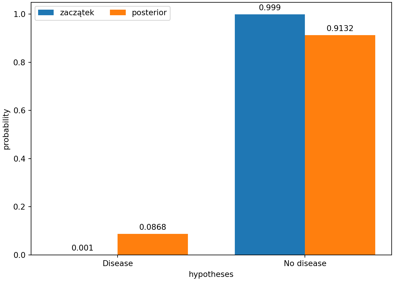
5.6 Zadania
Exercise 5.1 In a population, 0.1% of people are infected with a certain virus. If the virus is in the body, a test for the presence of the virus returns a positive result with a probability of 0.90, and a negative result with a probability of 0.10. In a situation where the virus is not in the body, the test returns a negative result with a probability of 0.99, and a positive (incorrect) result with a probability of 0.01. What is the probability that a randomly selected and tested person will have a positive test result for the presence of the virus?
Exercise 5.2 (Aczel and Sounderpandian 2018) The board of a holding company seeking to acquire a certain enterprise estimates the probability of acquisition at 0.65 if the board of the acquired enterprise resigns, and at 0.30 if the board of the acquired enterprise does not resign. The board of the holding company estimates the probability of the board of the acquired enterprise resigning at 0.70. What is the probability that the holding company will succeed in acquiring the enterprise?
Exercise 5.3 (McClave and Sincich 2012) 60% of the passengers at a small airport travel on major airlines, 30% travel on private planes, and the rest travel on non-major commercial planes. Of those traveling on major airlines, 50% travel on business; the percentage of business travelers among those traveling on private planes is 60%; among the rest, it is 90%. We randomly select one airport passenger. What is the probability that this person: (a) is traveling on business? (b) is traveling on business by private plane? (c) is traveling on private plane if we know that he or she is traveling on business? (d) is traveling on business if we know that he or she arrived on a commercial (non-private) plane?
Exercise 5.4 (Maddala 2006) This task is an illustration of the randomized response technique) which allows one to obtain an answer when one is not sure if the question has been asked at all.
We want to know the fraction of students who have tried drugs. A direct question may not give us honest answers. Instead, we give students a box containing 4 blue, 3 red, and 4 white balls. Each student is asked to draw (with replacement) a ball and follow the instructions that sayn:
- if a blue ball is drawn, answer the question “have you tried drugs”;
- if a red ball is drawn, say “yes”;
- if a white ball is drawn, say “no”.
The person asking the question does not see which ball was drawn by the student, so he or she is not sure if the student is answering the question or not..
Now, if 40% answered “yes”, what is the estimated percentage of students who have tried drugs?
Exercise 5.5 (Aczel and Sounderpandian 2018) A pollster wants to interview married couples about the usefulness of a certain product. He comes to a block of flats with three apartments. From the names on the mailboxes in the stairwell, he finds out that a married couple lives in one apartment, two men in the other, and two women in the third. However, it turns out that there are no numbers or names of the tenants on the doors of three apartments. Therefore, it is not known which of the three apartments the married couple lives in. The pollster chooses a door at random and rings the doorbell. The door is opened by a woman. In light of these facts, what is the probability that the pollster has found an apartment occupied by a married couple? (Assume that: if the apartment is occupied by two men, then a woman cannot open the door, if the apartment is occupied by two women, then only a woman can open the door, if the apartment is occupied by a married couple, then the probability of a woman opening the door is equal to 1/2. Also assume that a priori there is a 1/3 probability of finding an apartment occupied by a married couple).
Exercise 5.6 In a population, 0.1% of people are infected with a certain virus. If the virus is in the body, a test for the presence of the virus returns a positive result with a probability of 0.90, and a negative result with a probability of 0.10. In a situation where the virus is not in the body, the test returns a negative result with a probability of 0.99, and a positive (incorrect) result with a probability of 0.01. What is the probability that a randomly selected and tested person is infected with the virus if we know that the test gave a positive result?
Exercise 5.7 (Lee 2018) Suppose 40% of all emails are spam; 10% of spam emails contain the word “viagra”, while only 0.5% of non-spam emails contain the word “viagra”. What is the probability that an email is spam, given that it contains the word “viagra”?
Exercise 5.8 Fraudulent transactions constitute 0.035% of all payment card transactions. Among fraudulent transactions, 19.3% are transactions that are performed in locations geographically distant from the customer's place of residence. Among regular transactions, transactions in geographically distant places constitute only 0.4%.
What is the share of geographically distant transactions in all transactions?
A transaction is selected and found to have been performed in a location geographically distant from the customer's place of residence. What is the probability that this is a fraudulent transaction?
Exercise 5.9 Let's assume that PCR tests for COVID-19 had a sensitivity of 80% and a specificity of 98.5%. Let's assume that among people with cold symptoms at the time of the test, 30% had COVID, and in the entire population at that time one in a hundred people was infected with COVID.
What was the probability that a person drawn from among people with cold symptoms actually had COVID given their test was positive?
What was the probability that a person drawn from the entire population was actually infected with COVID if we know that their test was positive?
Exercise 5.10 (Based on Mcelreath 2020) Let's assume that there are two planets in a certain planetary system: “Earth” and “Mars”. “Earth” is covered by 70% water, 30% land, and “Mars” is 100% land. We land on one of the planets (let's assume that landing on each planet is equally likely), in a random location. We land on land. What is the probability that it is “Earth”?
Exercise 5.11 Some psychologists look for relationships between different behaviors using statistical tests. Only 1% of hypothetical relationships are true. If the relationship is false, statistical tests indicate that it is statistically significant 5% of the time. If the relationship is true, statistical tests detect it (indicate it as statistically significant) 80% of the time.
The relationship has been identified as significant by a statistical test. What is the probability that it is true?
What is the probability that one randomly selected and tested hypothetical relationship will be indicated as significant by a statistical test?
Exercise 5.12 Bogdan flew from Gdańsk to La Paz with two transfers and is currently waiting for his suitcase at the baggage claim. He knows that there is a 0.1% chance (1 in 1000) that his luggage could be lost. The luggage is placed on the belt evenly over a period of 10 minutes. After 8 minutes, most passengers have collected their luggage, but Bogdan's suitcase has not yet appeared. What is the probability that his suitcase has been lost?
Exercise 5.13 (Based on Mcelreath 2020) Assume there are two species of pandas. Both are equally common in the wild and live in the same areas. They look and feed exactly the same, but they differ in the frequency of twin births. Species A gives birth to twins in 10% of cases. Species B gives birth to twins in 20% of cases. Now, assume you are observing a female panda of an unknown species, and she has just given birth to twins.
What is the probability that this is a panda of species A?
What is the probability that the next birth will also be twins?
In the next birth, the same panda gave birth to a single cub. What is the probability now that this is a panda of species A?
Exercise 5.14 (Based on “Bayes’ Rule: Log-Odds Form,” n.d.) Janusz often travels to Alicante, where his friends Alejandro and Beatriz live. One of them always picks him up from the airport. Assume that both of them pick up Janusz equally often. They have two cars: a red one and a silver one. Beatriz prefers the red car; she uses the red car 60% of the time. Alejandro uses the silver car 4 times more often than the red one. Alejandro is more often late. If Alejandro picks up Janusz, the probability that he will be on time is 0.4; Beatriz will be on time with a probability of 0.8. Beatriz likes to use the horn. If she sees Janusz, she will honk 8 out of 10 times. Alejandro also sometimes uses the horn – the probability that he will honk when he sees Janusz is 0.2.
Janusz has just exited the arrivals hall and sees that a silver car is already waiting for him, and the driver is honking at him. What is the probability that it is Beatriz? Assume that using the horn, the color of the car, and being on time or late are independent of each other.