9 Continuous distributions

9.1 Density function

For continuous variables, instead of a probability mass function, we use a probability density function. The probability density function (PDF), most often denoted simply by the letter $f$, satisfies two conditions:

It is non-negative

\[ f(x) \ge 0 \text{ dla wszystkich x,} \tag{9.1}\]

The area under the density curve is 1 (probability of a certain event).

\[ \int_{-\infty}^{\infty}f(x) dx = 1 \tag{9.2}\]

We read off the probability by calculating the integral (i.e. determining the area under the curve)²:

\[ \mathbb{P}(a < X < b) = \int_{a}^{b}f(x)dx \tag{9.3}\]

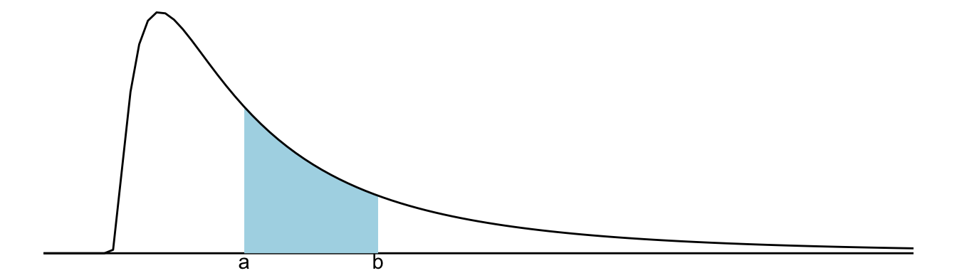
For a continuous variable, the probability that the variable will take on a value between a and b is equal to the area under the density curve over that segment

Figure 9.1: For a continuous variable, the probability that the variable will take on a value between a and b is equal to the area under the density curve over that segment

Mathematically, the area under a single point is infinitesimally small, meaning it is effectively zero. As a result, for continuous variables, the probability of any specific value $a$ is given by $\mathbb{P}(X=a) = 0$. While this may seem counterintuitive, it is logically consistent...

Hence, for continuous variables, the following equation holds:

\[ \mathbb{P}(a< X < b) = \mathbb{P}(a\le X \le b) = \mathbb{P}(a\le X < b) = \mathbb{P}(a < X \le b) \tag{9.4} \]

In other words, for continuous variables, whether we include the endpoints of an interval (closed interval) or exclude them (open interval) has no impact on the probability. In general, probabilities for a continuous random variable are only meaningful when calculated over intervals.

9.2 Uniform distribution

The continuous uniform distribution It is a distribution in which the density is uniform over a given interval (from $c$ to $d$).

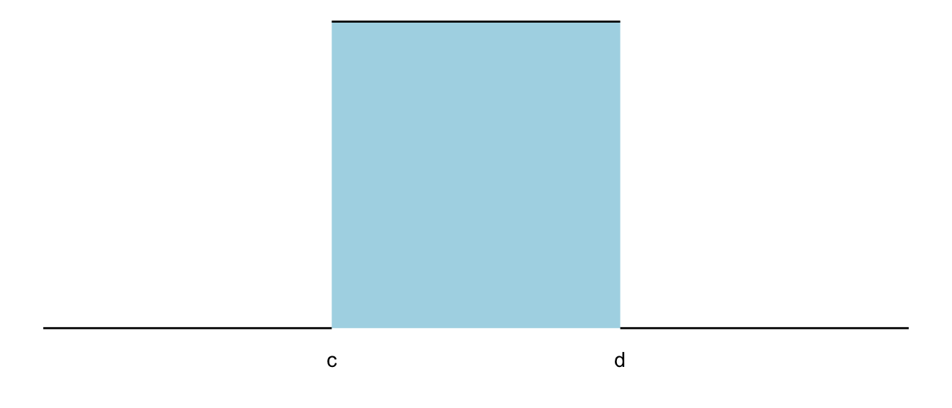
Figure 9.2: PDF of continuous density distribution

Since the area under the probability density function must equal 1, the value of the probability density function in the interval (c,d) is given by $f(x) = 1/(d-c)$.

Using the formulas (7.9) and (7.12), it can be shown that the mean of the uniform distribution is:

\[\begin{equation} \mu=\frac{c+d}{2}, \tag{9.5} \end{equation}\]

and the variance:

\[\begin{equation} \sigma^2= \frac{(d-c)^2}{12} \tag{9.6} \end{equation}\]

9.3 Gaussian distribution

The Gaussian distribution is usually referred to as the normal distribution. This does not mean that other distributions are abnormal—it is simply a name³.

The formula for the probability density function of this distribution (which we will not use explicitly, as integration will be handled by a computer) is:

\[ f(x)=\frac{1}{\sigma \sqrt{2 \pi}} e^{-\frac{(x-\mu)^2}{2 \sigma^2}}\:\:\:\:\:\:\: x \in \left(-\infty, \infty \right) \tag{9.7}\]

A random variable $X$ with a normal distribution, whose density function is given by equation (9.7), has a mean of $\mu$ and a variance of $\sigma^2$. This is denoted as:

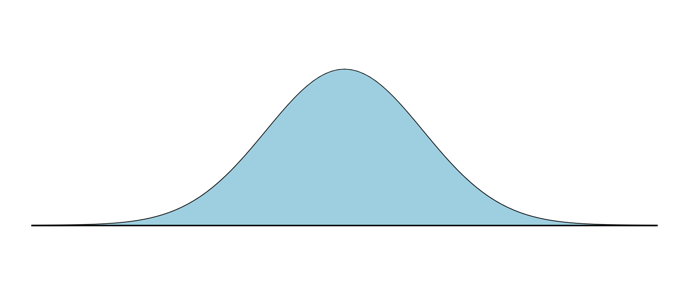
Figure 9.3: Shape of the density function of the normal distribution

9.3.1 Standardized normal distribution

A normal distribution generally has two parameters: the mean ($\mu$) and the standard deviation ($\sigma$). A normally distributed variable follows a standard (or standardized) normal distribution if $\mu=0$ and $\sigma=1$. The variable following the standardized Gaussian distribution is commonly denoted by $Z$: $Z \sim \mathcal{N}(0, 1)$.

A normally distributed variable $X$ with an expected value $\mu$ and a standard deviation $\sigma$ can be transformed into a standard normal variable $Z$ by subtracting the mean and dividing by the standard deviation:

\[ Z = \frac{X - \mu}{\sigma} \]

It is worth mentioning that any variable or list of data can be standardised. Standardisation (calculation of the standard score z-score) consists in transforming a variable or list according to the above rule (one subtracts the mean and divide the resulting difference by the standard deviation). Of course, standardisation performed in this way will not convert a variable with a non-normal distribution into a variable with a normal distribution.

9.3.2 Sum and difference of variables with normal distribution

If we have two independent variables X and Y with normal distributions with means $\mu_X$ and $\mu_Y$ and standard deviations $\sigma_X$ and $\sigma_Y$ respectively, then

the random variable X+Y has a normal distribution with mean $\mu_X+\mu_Y$ and standard deviation $\sqrt{\sigma^2_X+\sigma^2_Y}$,
the random variable X-Y has a normal distribution with mean $\mu_X-\mu_Y$ and standard deviation $\sqrt{\sigma^2_X+\sigma^2_Y}$.

The above formulae can be extended to more variables.

9.3.3 Approximation of binomial distribution by normal distribution

A binomial distribution with parameters $n$ and $p$ can be approximated by a normal distribution with mean $np$ and standard deviation $\sqrt{np(1-p)}=\sqrt{npq}$. Sometimes this is convenient and useful, and sometimes it may be necessary. The approximation works reasonably well if the tails of the normal distribution up to three sigma fall between the values $0$ and $n$, i.e:

\[ np - 3\sqrt{npq\vphantom{b}} > 0 \:\:\:\:\:\: \text{i} \:\:\:\:\:\: np + 3\sqrt{npq\vphantom{b}} < n\]

When we approximate the binomial distribution by means of the normal distribution, we often use the so-called continuity correction, that is, we assume that the value of the binomial variable $a$ corresponds to the area under the curve of the corresponding normal distribution over the segment $(a-0.5; a+0.5)$ – see figure 9.4.

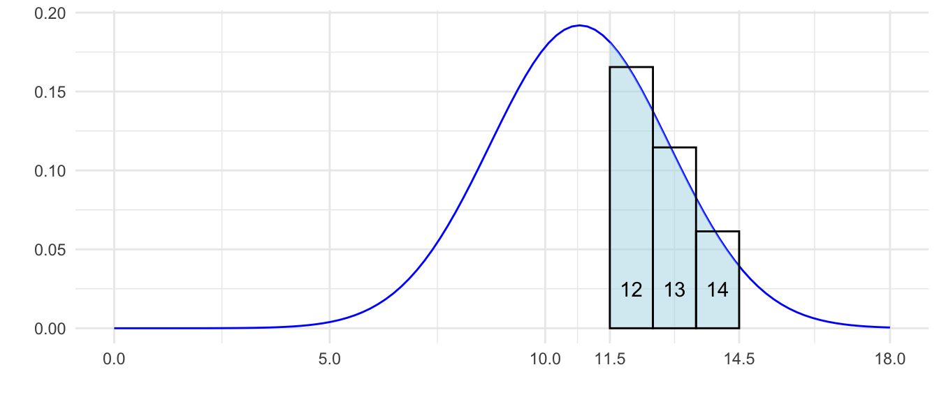
$The distribution of a variable with a binomial distribution can be approximated by a normal distribution with mean $np$ and standard deviation $\sqrt{npq}.$$

Figure 9.4: The distribution of a variable with a binomial distribution can be approximated by a normal distribution with mean $np$ and standard deviation $\sqrt{npq}.$

Wizualizacja przybliżenia rozkładu dwumianowego rozkładem normalnym: [https://college.cengage.com/nextbook/statistics/utts_13540/student/html/simulation8_4.html]

9.4 Templates

Spreadsheets

Normal distribution calculator — Google spreadsheet

Normal distribution calculator — Excel spreadsheet: Kalkulator_rozkladu_normalnego.xlsx

R code

##### 1. Area under PDF #####
# Gaussian distribution parameters:
# mean:
m <- 0
# standard deviation:
sd <- 2

# Calculating the area under PDF
# from
# *for minus infinity use from <- -Inf
from <- -Inf
# to
# *for plus infinity use to <- Inf
to <- 2

# Data validation, calculation
if (from > to) {
  # from > to error
  print("!!! _From_ cannot be greater than _to_ !!!")
} else {
  
  # Probability notation
  
  if (to==Inf) {
    p=paste0("P(X>", from, ")")
  } else if (from==-Inf) {
    p=paste0("P(X<", to, ")")
  } else {
    p=paste0("P(", from, "<X<", to, ")")
  }
  print(p)
  
  # Calculating the area for the given segment:
  result<-pnorm(to, m, sd)-pnorm(from, m, sd)
  print(result)
}

## [1] "P(X<2)"
## [1] 0.8413447

# Plot
library(ggplot2)

x1=if(from==-Inf){min(-4*sd+m, to-2*sd)} else {min(from-2*sd, -4*sd+m)}
x2=if(to==Inf){max(4*sd+m, from+2*sd)} else {max(to+2*sd, 4*sd+m)}

df<-data.frame(y=c(0, 0), 
               x=c(if(from==-Inf){NA}else{from}, if(to==-Inf){NA}else{to}),
               label=c(if(from==-Inf){NA}else{from}, if(to==-Inf){NA}else{to}))

plt<-ggplot(NULL, aes(c(x1, x2))) +
  theme_minimal() +
  xlab('') +
  ylab('') +
  geom_area(stat = "function", 
            fun = function(x){dnorm(x, m, sd)}, 
            fill = "orange", 
            xlim = c(if(from==-Inf){x1}else{from}, if(to==Inf){x2}else{to})) +
  geom_line(stat = "function", fun = function(x){dnorm(x, m, sd)}, col = "blue", lty=2, lwd=1) +
  scale_x_continuous(breaks=c(m, m-sd, m-2*sd, m+sd, m+2*sd, m-3*sd, m+3*sd, m-4*sd, m+4*sd)) +
  geom_point(data = df, aes(x=x, y=y), shape=4) +
  geom_text(data = df, aes(x=x, y=y, label=signif(label, 6)), vjust=1.4) +
  annotate("text", label = paste0("M = ", m, "\nSD = ", sd, "\n", p, " = ", signif(result,6)), 
           x = x1, y = dnorm(m, m, sd)*1.2, size = 6, hjust="inward", vjust = "inward")

suppressWarnings(print(plt))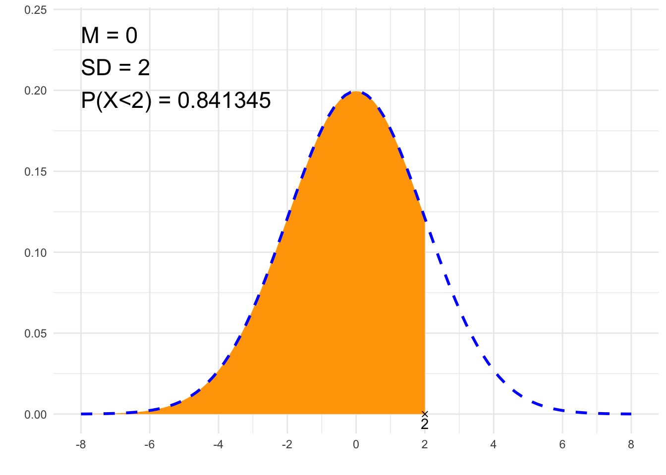

##### 2. Find x #####
# Gaussian distribution parameters:
# mean:
m <- 1
# standard deviation:
sd <- 3

# The area under PDF:
P <- 0.95

# 'L' - left, 'R' - right, 'S' - symmetrical (middle)
typ <- 'L'

# Calculations
from <- -qnorm(if(typ=='L'){1} else if(typ=='R'){P} else {1-(1-P)/2})*sd+m
to <- qnorm(if(typ=='L'){P} else if(typ=='R'){1} else {1-(1-P)/2})*sd+m

# P notation
if (to==Inf) {
  p=paste0("P(X>", signif(from, 6), ")")
} else if (from==-Inf) {
  p=paste0("P(X<", signif(to, 6), ")")
} else {
  p=paste0("P(", signif(from, 6), " < X < ", signif(to, 6), ")")
}
print(paste0(p, " = ", P))

## [1] "P(X<5.93456) = 0.95"

# Plot
library(ggplot2)

x1=if(from==-Inf){min(-4*sd+m, to-2*sd)} else {min(from-2*sd, -4*sd+m)}
x2=if(to==Inf){max(4*sd+m, from+2*sd)} else {max(to+2*sd, 4*sd+m)}

df<-data.frame(y=c(0, 0), 
               x=c(if(from==-Inf){NA}else{from}, if(to==-Inf){NA}else{to}),
               label=c(if(from==-Inf){NA}else{from}, if(to==-Inf){NA}else{to}))

plt<-ggplot(NULL, aes(c(x1, x2))) +
  theme_minimal() +
  xlab('') +
  ylab('') +
  geom_area(stat = "function", 
            fun = function(x){dnorm(x, m, sd)}, 
            fill = "orange", 
            xlim = c(if(from==-Inf){x1}else{from}, if(to==Inf){x2}else{to})) +
  geom_line(stat = "function", fun = function(x){dnorm(x, m, sd)}, col = "blue", lty=2, lwd=1) +
  scale_x_continuous(breaks=c(m, m-sd, m-2*sd, m+sd, m+2*sd, m-3*sd, m+3*sd, m-4*sd, m+4*sd)) +
  geom_point(data = df, aes(x=x, y=y), shape=4) +
  geom_text(data = df, aes(x=x, y=y, label=signif(label, 6)), vjust=1.4) +
  annotate("text", label = paste0("M = ", m, "\nSD = ", sd, "\n", p, " = ", P), 
           x = x1, y = dnorm(m, m, sd)*1.2, size = 6, hjust="inward", vjust = "inward")

suppressWarnings(print(plt))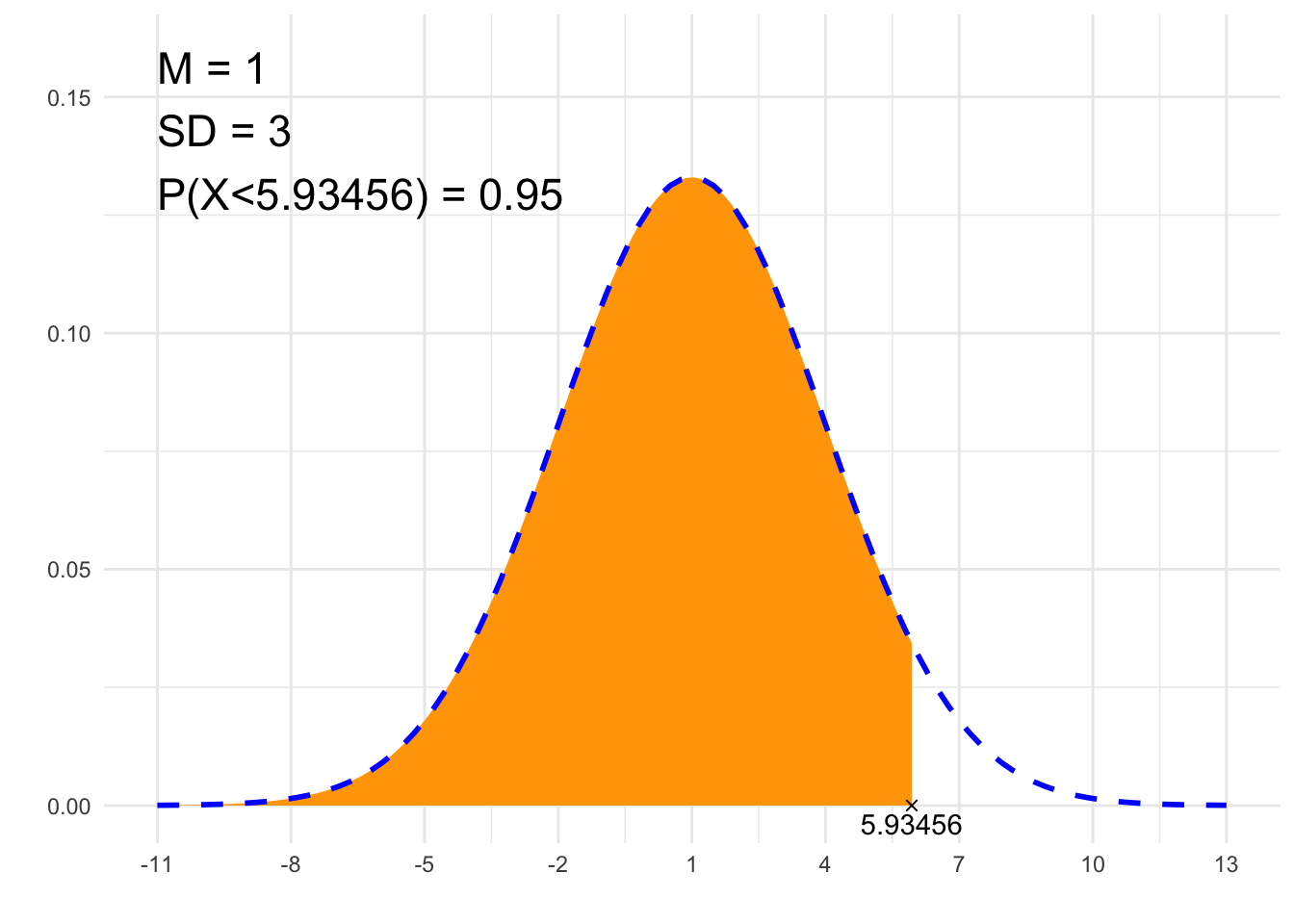

Kod w Pythonie

from scipy.stats import norm
##### 1. Area under PDF #####
# Gaussian distribution parameters:
# mean:
m = 0
# standard deviation:
sd = 2
# Calculating the area under PDF
# from
# *for minus infinity use _from = float('-inf')
_from = float('-inf')
# to
_to = 2

# Data validation, calculation
if _from > _to:
    print("!!! _From_ cannot be greater than _to_ !!!")
else:
    if _to == float('inf'):
        p = "P(X>" + str(_from) + ")"
    elif _from == float('-inf'):
        p = "P(X<" + str(_to) + ")"
    else:
        p = "P(" + str(_from) + "<X<" + str(_to) + ")"
    print(p)

    result = norm.cdf(_to, m, sd) - norm.cdf(_from, m, sd)
    print(result)

## P(X<2)
## 0.8413447460685429

##### 2. Find x #####

import numpy as np
from scipy.stats import norm

# Gaussian distribution parameters:
# mean:
m = 1
# standard deviation:
sd = 3

# The area under PDF:
P = 0.95

# 'L' - left, 'R' - right, 'S' - symmetrical (middle)
typ = 'L'

# Obliczenia
if typ == 'L':
    _from = -norm.ppf(1) * sd + m
    _to = norm.ppf(P) * sd + m
elif typ == 'R':
    _from = -norm.ppf(P) * sd + m
    _to = norm.ppf(1) * sd + m
else:
    _from = -norm.ppf(1-(1-P)/2) * sd + m
    _to = norm.ppf(1-(1-P)/2) * sd + m

# Zapis prawdopodobieństwa
if np.isinf(_to):
    p = f"P(X>{np.round(_from, 6)})"
elif np.isinf(_from):
    p = f"P(X<{np.round(_to, 6)})"
else:
    p = f"P({np.round(_from, 6)} < X < {np.round(_to, 6)})"
print(f"{p} = {P}")

## P(X<5.934561) = 0.95

9.5 Exercises

Exercise 9.1 The time required to complete a certain task has a uniform distribution in the interval [4, 10] minutes.

Write down the density function of this random variable.
What is the probability that the task will be completed in at most 8 minutes?
What is the expected time for the task to be completed?

Exercise 9.2 Kevin has just landed at the airport and is waiting in the baggage claim hall in front of the baggage carousel, which has just started moving. Let's assume that the belt will be in motion for 10 minutes, with the luggage being placed on the belt evenly throughout this period. What is the probability that Kevin's suitcase will appear on the belt within the first three minutes?

Exercise 9.3 A student commutes to university by metro. Trains arrive exactly every 12 minutes, but their arrival time is random. When planning his day, the student assumes a maximum waiting time of 8 minutes for the metro; if he waits longer, he will be late for class.

What is the expected waiting time for the metro? What is the variance?
What is the probability that the student will wait for the metro for more than four but no longer than six minutes?
What is the probability that the student will make it to class on time?
If the student wants to be 95% sure that he will arrive on time for class, how long can he wait for the metro at most?

Exercise 9.4 Let X have the following density function:

\[f(x) =\begin{cases} (x-5)/18 & \text{ dla } 5 \le x \le 11 \\ 0 & \text { dla pozostałych } \end{cases}\]

Sketch the graph of the density function.
Show that $f(x)$ is a density function.
What is the probability that X takes a value greater than 7?

Exercise 9.5 Quantiles (median, quartiles, percentiles) have their definition not only for real data but also for random variables. For example, the first quartile is the value $x_1$ of the random variable $X$ such that $\mathbb{P}(X<x_1)=0.25$. Find the median, first and third quartiles, interquartile range (IQR), fifth, tenth, ninetieth, and ninety-fifth percentiles of the standard normal distribution.

Exercise 9.6 (McClave and Sincich 2012) The time to failure of a certain printer (in hours) follows a normal distribution with a mean of 549 and a standard deviation of 68. Find the probability that the printer will operate without failure for at least 500 hours.

Exercise 9.7 (Aczel and Sounderpandian 2018) The power output generated by a solar battery is approximately normally distributed with a mean of 15.6 kilowatts and a standard deviation of 4.1 kilowatts. How many kilowatts will the battery generate at least with 95% confidence?

Exercise 9.8 Assume that the height distribution of patients is approximately normal with a mean of 175.9 cm and a standard deviation of 9.0 cm. What size must a bed be to accommodate 99.5% of patients?

Exercise 9.9

(Aczel and Sounderpandian 2018) The GMAT exam scores of students considering applying to university are approximately normally distributed with a mean of 487 points and a standard deviation of 98 points.

What percentage of students will score above 500?
What percentage of students will score between 600 and 700?
If the university wants to allow only the top 75% of students to apply, what should be the cutoff, minimum GMAT score?
Find the narrowest interval that will contain the scores of 75% of students.

Exercise 9.10 (McClave and Sincich 2012) Scientists have determined that the length of the shells of green sea turtles in one of the lagoons on Grand Cayman Island has (approximately) a normal distribution with a mean of 55.7 cm and a standard deviation of 11.5 cm.

Only turtles with shells longer than 40 cm and shorter than 60 cm can be legally caught. What is the probability of catching a turtle with illegal dimensions?

What is the maximum limit L such that after setting it, only 10% of the caught turtles will exceed this limit?

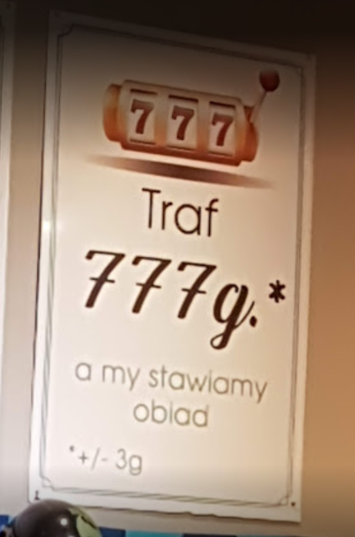
Exercise 9.11 A few years ago, a food bar at Gdańsk Politechnika station offered a free meal if the weight showed 777 ± 3 grams. What was the probability of randomly receiving a free meal if the distribution of the weight of the portions served by the customers was normal with a mean of 620 grams and a standard deviation of 130 grams?

Exercise 9.12 (Utts and Heckard 2014) Meg travels frequently and has recently started to take risks when it comes to making sure she has enough time to get to the airport. She leaves home 45 minutes before the last call for her flight. Her travel time from her flat door to the airport car park has a normal distribution with an average of 25 minutes and a standard deviation of 3 minutes. From the car park she then has to take a shuttle bus to the terminal and go through security. The average time to do this is 15 minutes with a standard deviation of 2 minutes, and this time also has a normal distribution. The time to get there and the time at the airport are independent of each other. What is the probability that Meg will miss her flight because her total time to get to the airport will exceed 45 minutes?

Exercise 9.13 (Utts and Heckard 2014) Can Alison win over her sister? Alison and her sister Julie swim a mile every day. Alison's times have a normal distribution with mean = 37 minutes and standard deviation = 1 minute. Julie is faster, but her times are less uniform than Alison's results: they have a normal distribution with mean = 33 minutes and standard deviation = 2 minutes. Each day their results are independent of each other. Will Alison ever beat Julie? What is the probability of such an event?

Exercise 9.14 What is the probability that in 1000 tosses of a 'fair' coin, we get heads more than 550 times? The answer should be given by approximating the binomial distribution with a normal distribution.

Exercise 9.15 What is the probability that in a trillion tosses of a 'fair' coin, we get heads less than 499999 million times? The answer should be given by approximating the binomial distribution with a normal distribution.

Exercise 9.16 (Maddala 2006) The probability density function of the continuous random variable X is given by:

\[f(x) =\begin{cases} kx(2-x) & \text{ for } 0 \le x \le 2 \\ 0 & \text { otherwise } \end{cases}\]

Find $k$.
Compute $\mathbb{E}(X)$ i $\mathbb{V}(X)$.
Find the probability that X will be less than 0.5.

Exercise 9.17 (Maddala 2006) The probability density function of the continuous random variable X is given by:

\[f(x) =\begin{cases} kx & \text{ for } 0 \le x \le 1 \\ k(2-x) & \text{ for } 1 < x \le 2 \\ 0 & \text { otherwise } \end{cases}\]

Find $k$.
Compute $\mathbb{E}(X)$ i $\mathbb{V}(X)$.
Find the probability that X will be less than 0.5.

Exercise 9.18 The teacher graded the tests and realized that two tests (the first graded 80/100 and the second graded 45/100) are not signed. Based on the attendance list, he could determine that they belong to Alek and Bolek. Based on the previous work of these students, he would expect Alek's score to be around 75 plus/minus 12 points, and Bolek's score to be around 60 points plus/minus 20. Assuming normal distributions in both cases (for Alek with a mean of 75 and a standard deviation of 12 points, for Bolek with a mean of 60 and a standard deviation of 20 points), calculate the probability that the first test is Alek's and the second test is Bolek's.

Literature

Aczel, A. D., and J. Sounderpandian. 2018. Statystyka w Zarządzaniu. PWN. https://ksiegarnia.pwn.pl/Statystyka-w-zarzadzaniu,731934758,p.html.

Maddala, G. S. 2006. Ekonometria. Wydawnictwo Naukowe PWN.

McClave, J. T., and T. T. Sincich. 2012. Statistics. Pearson Education. https://books.google.pl/books?id=gcYsAAAAQBAJ.

Utts, Jessica M., and Robert F. Heckard. 2014. Mind on Statistics - Standalone Book. 5th edition. Australia; United States: Brooks Cole.

In practice, for continuous variables, we often use the CDF $F_X$: \[ \mathbb{P}(a < X < b) = P(X \le b) - P(X \le a) = F_X(b)-F_X(b) =\int_{-\infty}^{b}f(x)dx-\int_{-\infty}^{a}f(x)dx \]↩︎
Just like the expected value is not necessarily what one expects, and a success in the binomial distribution is not necessarily a success…↩︎