21 Linear regression
21.1 Linear regression model – assumptions
In statistics, a model is often defined as an assumption that the data in a sample have been generated by a probabilistic process belonging to a specific group of processes12.
The linear regression model assumes that the process by which the data were generated can be described by the following equation:
\[y_i = \beta_0 + \beta_1 \times x_i + \varepsilon_i, \tag{21.1}\]
in the case of simple regression (where there is only one explanatory variable),
or by the following:
\[y_i = \beta_0 + \beta_1 x_{i1} + \beta_2 x_{i2} + \dots + \beta_k x_{ik} + \varepsilon_i, \tag{21.2}\]
when there are \(k\) explanatory variables (\(k>1\)) – multiple regression.
Thus, it is assumed that the relationship between the explanatory variables (denoted by X) and the dependent variable (denoted by Y) is linear.
The regression model equations include a random component, \(\varepsilon_i\), which is typically assumed to satisfy the following conditions:
Its expected value is always zero: \(\mathbb{E}(\varepsilon_i)=0\).
Its variance is constant (does not depend on X or any other factors) and equals \(\sigma_\varepsilon^2\) (the assumption of constant variance in this context is called homoscedasticity13).
Its values are generated without autocorrelation (i.e. the value of the random component for any observation \(i\) is not correlated with the value of the random component for any other observation \(j\)).
Its values follow a normal distribution.
As a result, the classical linear regression model assumes that the conditional distribution \(Y_i|\left(X_1=x_{i1}, X_2=x_{i2}, \dots X_k=x_{ik}\right)\) is a Gaussian distribution with an expected value of:
\[\mu_{y_i} = \beta_0 + \beta_1 x_{i1} + \beta_2 x_{i2} + \dots + \beta_k x_{ik} \tag{21.3}\]
and a standard deviation of \(\sigma_\varepsilon\).
Figure 21.1: A regression model is a model of the conditional distribution of the dependent variable – an example using a simulated relationship between the number of study hours and exam scores.
21.2 Linear regression model – estimation
The values of \(\beta_0\), \(\beta_1\), ..., \(\beta_k\), and \(\sigma_\varepsilon\) are unobserved parameters of the data-generating process (the "population"), which can be estimated based on a random sample.
In the case of the classical linear regression model, the \(\beta\) coefficients are estimated using the least squares estimator.
For simple regression, the estimator of the slope coefficient (\(\beta_1\)) can be expressed as:
\[ \widehat{\beta}_1 = \frac{\sum_{i=1}^{n} (x_i - \bar{x})(y_i - \bar{y})}{\sum_{i=1}^{n} (x_i - \bar{x})^2}, \tag{21.4} \]
while the formula for the estimator of the intercept is:
\[ \widehat{\beta}_0 = \bar{y} - \widehat{\beta}_1 \bar{x}. \tag{21.5} \]
For multiple regression, the least squares estimator in matrix notation takes the following form:
\[\widehat{\boldsymbol{\beta}}=\left(\mathbf{X}^\top\mathbf{X}\right)^{-1}\mathbf{X}^\top \mathbf{y}, \tag{21.6} \]
where \(\widehat{\boldsymbol{\beta}}\) is the column vector of estimated coefficients \(\beta_0, \dots, \beta_k\) (\(k\) being the number of explanatory variables), \(\mathbf{X}\) is the design matrix, which consists of rows corresponding to individual observations and columns corresponding to explanatory variables (including a column of ones for the intercept term), and \(\mathbf{y}\) is the column vector of dependent variable values.
The parameter \(\sigma\) is estimated using the following formula:
\[ \widehat{\sigma}_\varepsilon = \sqrt{\widehat{\sigma}_\varepsilon^2} \tag{21.7} \]
\[ \widehat{\sigma}_\varepsilon^2 = \frac{\sum_i(y_i-\hat{y}_i)^2}{n-k-1} \tag{21.8} \]
Estimation is typically carried out using statistical software.
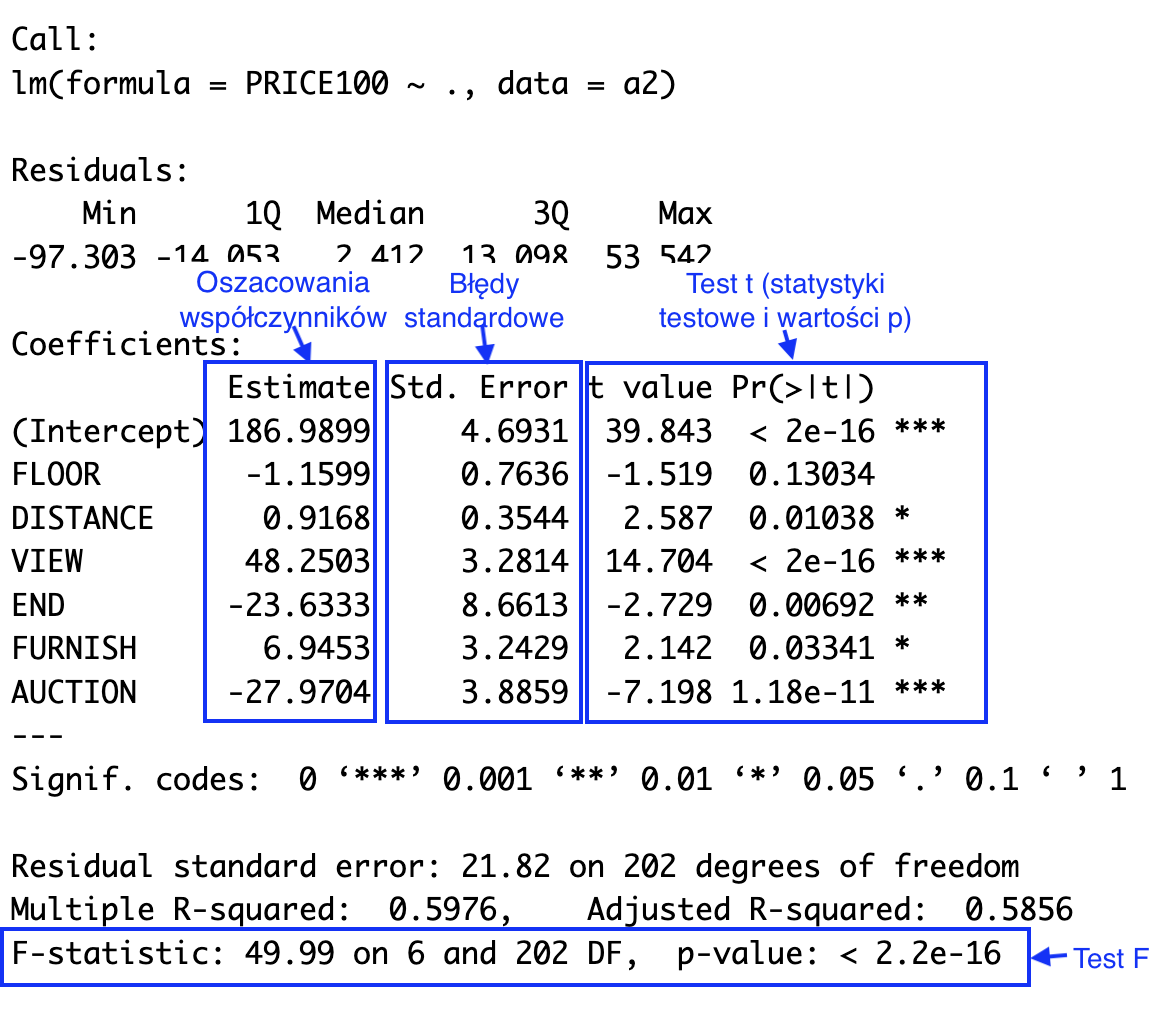
Figure 21.2: Typical linear regression summary in R
21.2.1 Confidence intervals for model coefficients
The confidence interval for the model coefficient \(\beta_j\) (\(j = 1, 2, \dots, p\)) can be determined using the following formula:
\[\widehat{\beta}_j \pm t_{\alpha/2} \times \widehat{SE}(\widehat{\beta}_j), \tag{21.9}\]
where \(\widehat{\beta}_j\) is the point estimate of the coefficient \(\beta_j\), \(\widehat{SE}(\widehat{\beta}_j)\) is the estimated standard error of this coefficient’s estimator, and \(t_{\alpha/2}\) is the corresponding quantile from the t-Student distribution with \(n - p - 1\) degrees of freedom (\(n\) is the number of observations in the sample, and \(p\) is the number of explanatory variables).
The formulas for calculating the standard error in simple regression are as follows. For the slope coefficient (\(\beta_1\)):
\[ \widehat{SE}(\widehat{\beta}_1) = \frac{\widehat{\sigma}_\varepsilon}{\sqrt{\sum_i (x_i - \bar{x})^2}} \tag{21.10}\]
and for the intercept term:
\[ \widehat{SE}(\widehat{\beta}_0) = \widehat{\sigma}_\varepsilon \sqrt{\frac{1}{n} + \frac{\bar{x}^2}{\sum_i (x_i - \bar{x})^2}} \tag{21.11}\]
In multiple regression, standard error estimates are obtained using the following matrix algebra-based formula:
\[\widehat{SE}(\widehat{\beta}_j) = \widehat{\sigma}_\varepsilon \sqrt{\left[\left( \mathbf{X}^\top\mathbf{X}\right)^{-1} \right]_{jj}}, \tag{21.12}\]
where \(\mathbf{A}_{jj}\) represents the element of matrix \(\mathbf{A}\) located in the \(j\)-th row and \(j\)-th column.
In practice, standard errors are calculated by statistical software packages.
21.2.2 Confidence intervals for the expected value of the dependent variable
Confidence intervals for the conditional mean (expected conditional value) of the dependent variable, given fixed values of the explanatory variables, are determined using the following formula:
\[\widehat{y}_h \pm t_{\alpha/2} \times \widehat{SE}(\widehat{y}_h), \tag{21.13}\]
where \(x_{h1}, \dots, x_{hp}\) are fixed values of the explanatory variables, which can be arranged into a column vector \(\mathbf{x}_h\). The term \(\hat{y}_h = \hat{\beta_0} + \hat{\beta_1} x_{h1} + \dots + \hat{\beta_k} x_{hk}\) represents the point estimate of the expected value of \(Y\) in this scenario, and \(\widehat{SE}(\hat{y}_h)\) is the estimate of its standard error.
For simple regression:
\[ \widehat{SE}(\hat{y}_h) = \widehat{\sigma}_\varepsilon\sqrt{\frac{1}{n}+\frac{(x_h-\bar{x})^2}{\sum_i(x_i-\bar{x})^2}}, \tag{21.14} \]
and for multiple regression:
\[\widehat{SE}(\hat{y}_h) = \widehat{\sigma}_\varepsilon\sqrt{\mathbf{x}_h^\top (\mathbf{X}^\top\mathbf{X})^{-1}\mathbf{x}_h}. \tag{21.15}\]
21.3 Prediction intervals
Usually, we are interested not only in the expected value but also in the variability around this value. A prediction interval accounts for both of these aspects, as it provides an estimate of the range within which a new single observation from the same population (generated by the same process) is likely to fall with a given probability of \(1 - \alpha\).
For simple regression, the prediction interval is given by the following formula:
\[ \hat{y}_h\pm t_{\alpha/2}\widehat{\sigma}_\varepsilon\sqrt{1+\frac{1}{n}+\frac{(x_h-\bar{x})^2}{\sum_i(x_i-\bar{x})^2}}, \tag{21.16} \]
where \(\hat{y}_h\) is the expected value of the dependent variable \(Y\) given that the explanatory variable \(X\) is equal to \(x_h\).
For multiple regression, the following matrix-based formula can be used:
\[ \hat{y}_h\pm t_{\alpha/2}\widehat{\sigma}_\varepsilon\sqrt{1+\mathbf{x}_h^\top (\mathbf{X}^\top\mathbf{X})^{-1}\mathbf{x}_h} \tag{21.17} \]
21.4 Linear regression model – t-test and F-test
Statistical software packages (and even spreadsheet tools such as Excel) typically compute statistics that allow for two types of hypothesis tests in linear regression: tests for the significance of individual coefficients \(\beta_j\) (“t-tests”) and an overall model significance test (“F-test”).
21.4.1 Significance tests for coefficients
1. In the t-test for a coefficient \(\beta_j\), the null hypothesis states that it is equal to zero:
\[ H_0: \beta_j = 0 \]
2. The alternative hypothesis is two-sided:
\[ H_A: \beta_j \ne 0 \]
3. The test statistic is calculated as follows:
\[t = \frac{\widehat{\beta}_j}{\widehat{SE}(\widehat{\beta}_j)} \tag{21.18} \]
Under the null hypothesis, the test statistic follows a t-distribution with \(n - p - 1\) degrees of freedom.
4. The rejection region and p-value are determined in the same way as for other two-sided t-tests.
21.4.2 F-Test
1. In the F-test, the null hypothesis states that all explanatory variable coefficients are equal to zero:
\[ H_0: \beta_1 = \dots = \beta_k = 0 \]
It is important to note that the null hypothesis does not include the intercept term (\(\beta_0\)).
2. The alternative hypothesis states that at least one of them is different from zero:
\[ H_A:\text {istnieje } j \in \{1, \dots, k\}\text{, takie że } \beta_j \ne 0 \]
3. The test statistic follows an F-distribution with degrees of freedom in the numerator (\(df_1\)) equal to \(k\) and degrees of freedom in the denominator (\(df_2\)) equal to \(n - k - 1\):
\[ F_{(k,n-k-1)}=\frac{SSR/k}{SSE/(n-k-1)}=\frac{\sum_{i=1}^n\left(\widehat{y}_i-\bar{y}\right)^2/k}{\sum_{i=1}^n\left(y_i-\widehat{y}_i\right)^2/({n-k-1})} \tag{21.19} \]
21.5 Diagnostic tests for the regression model
It is important to remember that the assumptions of the linear regression model are almost always only approximately met in practice. Therefore, the main concern is not rejecting the null hypothesis (regarding linearity, normality, etc.), but rather assessing whether the deviation from the assumptions is substantial or minor.
Significance tests, however, answer a different question: if the data-generating process perfectly followed the model’s assumptions, how likely would it be to obtain the observed results or even more extreme ones?
(...)
Thus, diagnostic tests should be considered as auxiliary tools and will rarely serve as the sole criterion for decision-making.
21.5.1 Testing linearity
One way to assess linearity is through visual inspection, such as plotting residuals against fitted values or explanatory variables. If the relationship is not linear, patterns may appear in the residuals.
The most popular statistical test for linearity is Ramsey's RESET test. It examines whether non-linear combinations of explanatory variables significantly improve the model.
21.5.2 Testing homoskedasticity
Heteroskedasticity can be detected using residual plots. For example, if visual inspection suggests that the variance increases or decreases systematically with fitted values, heteroskedasticity may be present.
Popular statistical tests for homoskedasticity are Breusch-Pagan test and White’s test .
21.5.3 Testing normality of the error term
The assumption of normally distributed residuals is crucial mainly for hypothesis testing and confidence interval estimation. If residuals deviate significantly from normality, t-tests and F-tests may not be valid.
Visual inspection of Q-Q plots or histograms may reveal substantial deviations from normality.
Statistical tests for normality, such as Shapiro-Wilk test or Jarque-Bera test may be used on residuals to check normality of the error term.
21.6 Templates
Simple regression — Google spreadsheet
Simple regression — Excel template
Multiple regression — Google spreadsheet
Multiple regression — Excel template