22 Other tests
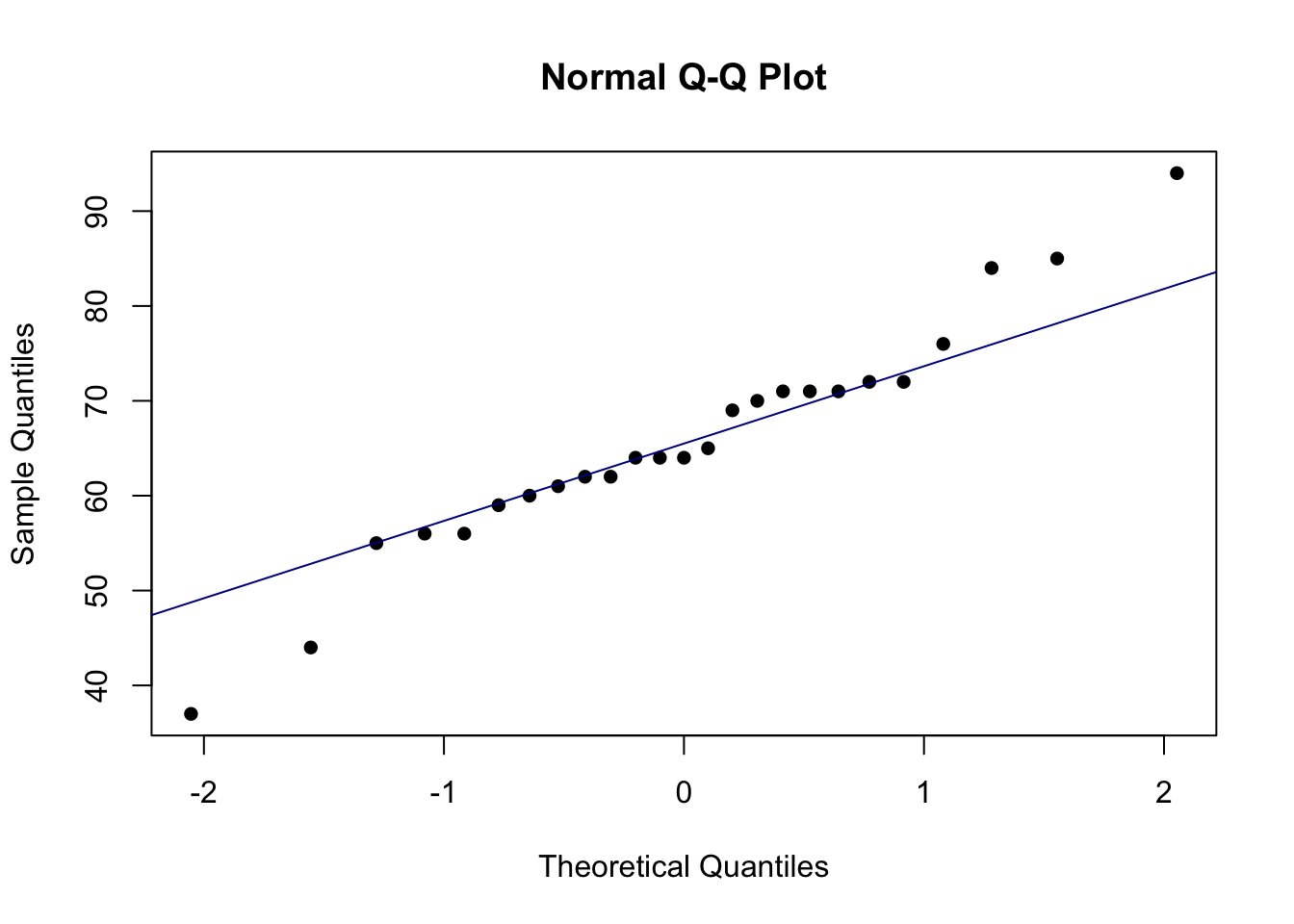
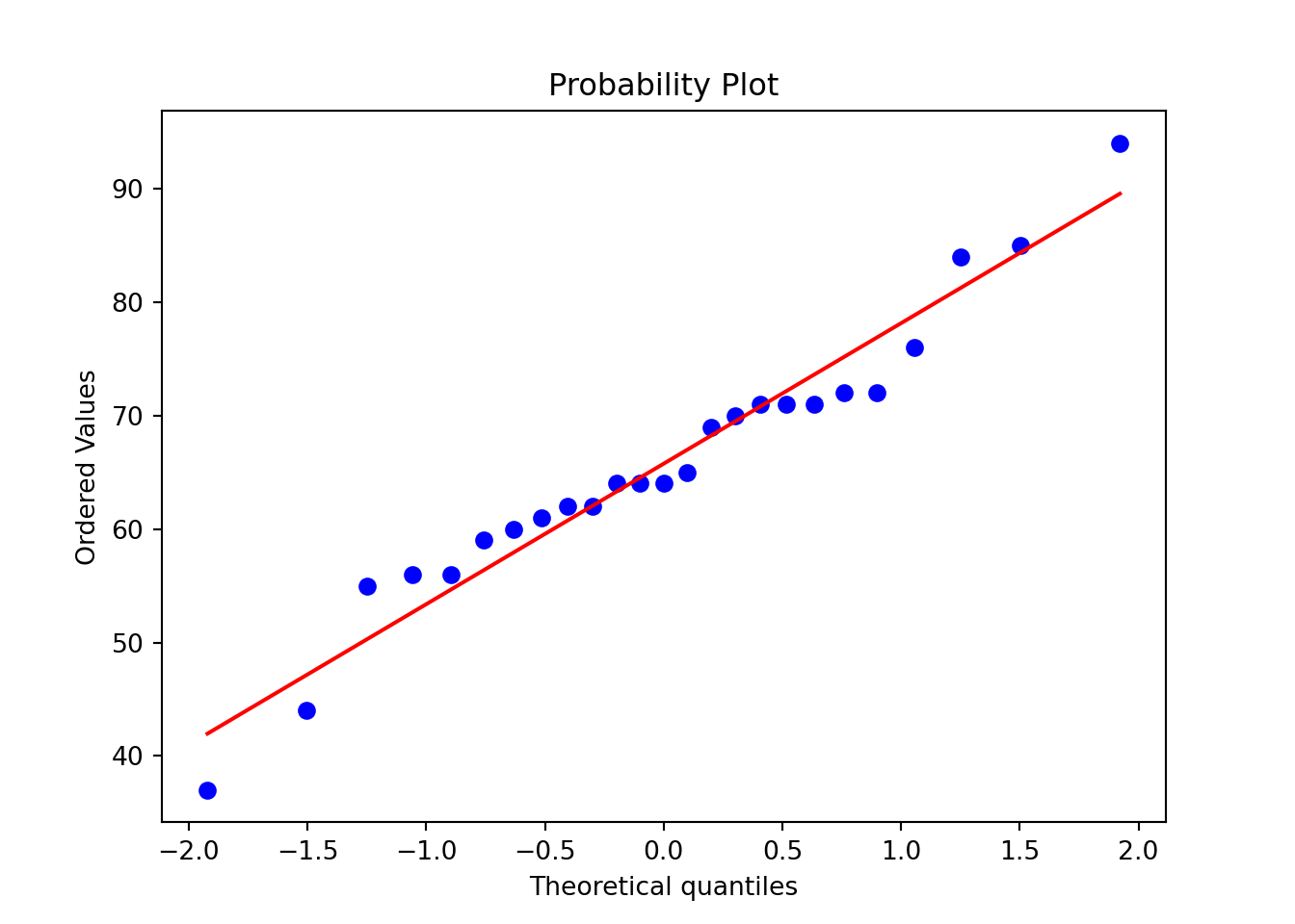
22.1 Checking conformity with the Gaussian distribution
Popular "normality tests" include the Kolmogorov-Smirnov test, the Shapiro-Wilk-Royston test, and the Jarque-Bera test.
22.2 Test and confidence interval for Pearson's correlation coefficient
The correlation coefficient examines the relationship between two quantitative variables. It can be positive or negative, and takes values between -1 and 1. The sample correlation coefficient is commonly denoted by the symbol \(r\), while the population correlation coefficient is represented by the Greek letter \(\rho\) ("rho").
A popular test for the correlation coefficient is the t-test. This test usually assumes that the joint probability distribution of the two variables follows a bivariate normal distribution.
The null hypothesis in this test states that the variables in the population are not linearly correlated:
\[ H_0: \rho = 0, \]
while the alternative hypothesis (two-tailed) states that they are linearly correlated:
\[ H_A: \rho \ne 0 \]
It is also possible to apply one-tailed hypotheses: \(H_A: \rho > 0\) lub \(H_A: \rho < 0\).
The test statistic is based on the \(t\) -distribution with \(n-2\) degrees of freedom and has the following form:
\[ t = r {\sqrt {\frac {n-2}{1-r^{2}}}}, \] where \(n\) is the sample size, and \(r\) is the correlation coefficient in the sample.
The formula for the confidence interval of Pearson's correlation coefficient is quite complex. The lower bound is obtained as follows:
\[ \frac{\text{exp}\left(ln\frac{1+r}{1-r}-\frac{2}{\sqrt{n-3}}z_{\alpha/2}\right)-1}{\text{exp}\left(ln\frac{1+r}{1-r}-\frac{2}{\sqrt{n-3}}z_{\alpha/2}\right)+1} \]
and the upper (right) bound is:
\[ \frac{\text{exp}\left(ln\frac{1+r}{1-r}+\frac{2}{\sqrt{n-3}}z_{\alpha/2}\right)-1} {\text{exp}\left(ln\frac{1+r}{1-r}+\frac{2}{\sqrt{n-3}}z_{\alpha/2}\right)+1} \]
22.3 Templates
Normality check — Google spreadsheet
Normality check — Excel template
Correlation coefficient — Google spreadsheet
Correlation coefficient — Excel template
R code
# Normality check
# Data
data<-c(76, 62, 55, 62, 56, 64, 44, 56, 94, 37, 72, 85, 72, 71, 60, 61, 64, 71, 69, 70, 64, 59, 71, 65, 84)
# Sample mean
m<-mean(data)
# Sample standard deviation
s<-sd(data)
# Skewness
skew<-e1071::skewness(data, type=2)
# Kurtosis
kurt<-e1071::kurtosis(data, type=2)
# IQR/s ratio
IQR_to_s<-IQR(data)/s
# proportion of observations within 1 sd from the mean
within1s<-mean(abs(data-m)<s)
# proportion of observations within 2 sds from the mean
within2s<-mean(abs(data-m)<2*s)
# proportion of observations within 3 sd from the mean
within3s<-mean(abs(data-m)<3*s)
# Shapiro-Wilk test
SW_res<-shapiro.test(data)
# Jarque-Bera test
JB_res<-tseries::jarque.bera.test(data)
# Anderson-Darling test
AD_res<-nortest::ad.test(data)
# Kolmogorov-Smirnov test
KS_res <- ks.test(data, function(x){pnorm(x, mean(data), sd(data))})

# Results
print(c('Mean' = m,
        'St. deviation' = s,
        'Sample size' = length(data),
        'Skewnes (~=0?)' = skew,
        'Kurtosis (~=0?)' = kurt,
        'IQR/s (~=1,3?)' = IQR_to_s,
        '68% rule' = within1s*100,
        '95% rule' = within2s*100,
        '100% rule' = within3s*100,
        'Test stat. - SW test' = SW_res$statistic,
        'P-value - SW test' = SW_res$p.value,
        'Test stat. - JB test' = JB_res$statistic,
        'P-value - JB test' = JB_res$p.value,
        'Test stat. - AD test' = AD_res$statistic,
        'P-value - AD test' = AD_res$p.value,
        'Test stat - KS test' = KS_res$statistic,
        'P-value - KS test' = KS_res$p.value
))
## Mean St. deviation Sample size Skewnes (~=0?)
## 65.760000000 12.145918382 25.000000000 -0.002892879
## Kurtosis (~=0?) IQR/s (~=1,3?) 68% rule 95% rule
## 1.121315636 0.905654036 80.000000000 92.000000000
## 100% rule Test stat. - SW test.W P-value - SW test Test stat. - JB test.X-squared
## 100.000000000 0.964892812 0.520206266 0.479578632
## P-value - JB test Test stat. - AD test.A P-value - AD test Test stat - KS test.D
## 0.786793609 0.445513641 0.260454333 0.143712404
## P-value - KS test
## 0.680154210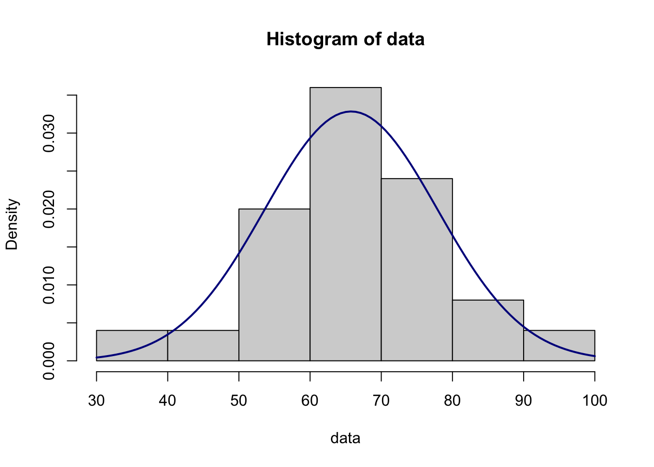
#data:
x <- c(4, 8, 6, 5, 3, 8, 6, 5, 5, 6, 3, 3, 3, 7, 3, 6, 4, 4, 8, 7)
y <- c(4, 6, 8, 3, 4, 6, 5, 8, 1, 4, 4, 3, 1, 6, 7, 5, 4, 4, 9, 5)
#test and confidence interval:
cor.test(x, y, alternative = "two.sided", conf.level = 0.95)
##
## Pearson's product-moment correlation
##
## data: x and y
## t = 2.56, df = 18, p-value = 0.01968
## alternative hypothesis: true correlation is not equal to 0
## 95 percent confidence interval:
## 0.09607185 0.78067292
## sample estimates:
## cor
## 0.5166288Python code
import numpy as np
import math as math
from scipy import stats
from scipy.stats import skew, kurtosis, anderson, kstest, norm

data = [76, 62, 55, 62, 56, 64, 44, 56, 94, 37, 72, 85, 72, 71, 60, 61, 64, 71, 69, 70, 64, 59, 71, 65, 84]

m = np.mean(data)

s = np.std(data, ddof=1)

skew = skew(data, bias=False)

kurt = kurtosis(data, bias=False)

IQR_to_s = stats.iqr(data) / s

within1s = np.mean(np.abs(data - m) < s)

within2s = np.mean(np.abs(data - m) < 2 * s)

within3s = np.mean(np.abs(data - m) < 3 * s)

SW_res = stats.shapiro(data)

JB_res = stats.jarque_bera(data)

AD_res = stats.anderson(data)

AD2 = AD_res[0]*(1 + (.75/50) + 2.25/(50**2))

if AD2 >= .6:
    AD_p = math.exp(1.2937 - 5.709*AD2 - .0186*(AD2**2))
elif AD2 >=.34:
    AD_p = math.exp(.9177 - 4.279*AD2 - 1.38*(AD2**2))
elif AD2 >.2:
    AD_p = 1 - math.exp(-8.318 + 42.796*AD2 - 59.938*(AD2**2))
else:
    AD_p = 1 - math.exp(-13.436 + 101.14*AD2 - 223.73*(AD2**2))

KS_res = kstest(data, norm(loc=np.mean(data), scale=np.std(data)).cdf)

results = {
    'Mean': m,
    'St. deviation': s,
    'Sample size': len(data),
    'Skewness (~=0?)': skew,
    'Excess kurtosis (~=0?)': kurt,
    'IQR/s (~=1.3?)': IQR_to_s,
    '68% rule': within1s * 100,
    '95% rule': within2s * 100,
    '100% rule': within3s * 100,
    'Test stat. - SW test': SW_res[0],
    'P-value - SW test': SW_res[1],
    'Test stat. - JB test': JB_res[0],
    'P-value - JB test': JB_res[1],
    'Test stat. - AD test': AD_res[0],
    'P-value - AD test': AD_p,
    'Test stat. - KS test': KS_res[0],
    'P-value - KS test': KS_res[1]
}


for key, value in results.items():
    print(f"{key}: {value}")
## Mean: 65.76
## St. deviation: 12.145918381634768
## Sample size: 25
## Skewness (~=0?): -0.002892878582795321
## Excess kurtosis (~=0?): 1.121315636006976
## IQR/s (~=1.3?): 0.9056540357320815
## 68% rule: 80.0
## 95% rule: 92.0
## 100% rule: 100.0
## Test stat. - SW test: 0.9648927450180054
## P-value - SW test: 0.5202044248580933
## Test stat. - JB test: 0.47957863171421605
## P-value - JB test: 0.7867936085428064
## Test stat. - AD test: 0.44551364110243696
## P-value - AD test: 0.27208274566708046
## Test stat. - KS test: 0.14001867878746022
## P-value - KS test: 0.6601736174333425import matplotlib.pyplot as plt
# Histogram
plt.hist(data, density=True)
xmin, xmax = plt.xlim()
x = np.linspace(xmin, xmax, 100)
p = stats.norm.pdf(x, m, s)
plt.plot(x, p, 'k', linewidth=2, color="darkblue")
plt.show()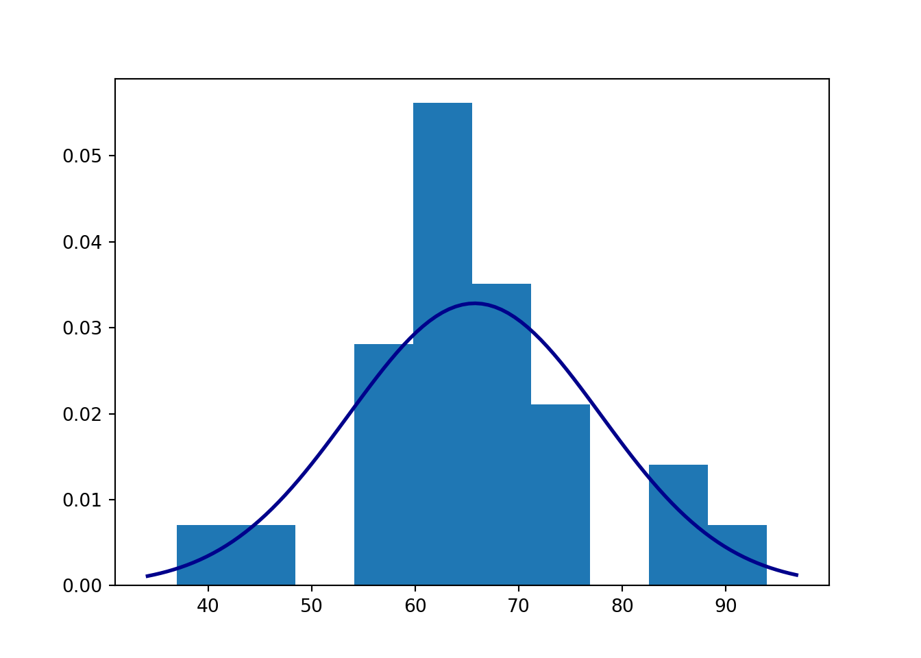
import scipy.stats as stats
import numpy as np

x = [4, 8, 6, 5, 3, 8, 6, 5, 5, 6, 3, 3, 3, 7, 3, 6, 4, 4, 8, 7]
y = [4, 6, 8, 3, 4, 6, 5, 8, 1, 4, 4, 3, 1, 6, 7, 5, 4, 4, 9, 5]

correlation_test = stats.pearsonr(x, y)

# Confidence interval:
ci_tmp = stats.norm.interval(0.95,
  loc=0.5*math.log((1+correlation_test[0])/(1-correlation_test[0])),
  scale=1/((len(x)-3)**0.5))
confidence_interval = (np.exp(2*np.array(ci_tmp))-1)/(np.exp(2*np.array(ci_tmp))+1)

print('Test:\n\n', correlation_test, '\n\n Confidence interval: \n\n', confidence_interval)
## Test:
##
## PearsonRResult(statistic=0.5166287822129882, pvalue=0.01968490591016886)
##
## Confidence interval:
##
## [0.09607185 0.78067292]22.4 Zadania
Exercise 22.1 30 students attempted to guess the age of a certain person based on a photograph. Each student provided their estimate. Treat these 30 students as a random sample from a population we wish to make inferences about. Should we reject the null hypothesis stating that the distribution of numbers provided by the students as estimates of the person’s age on the photo follows a Gaussian distribution?
Here are the numbers provided by the 30 students: 35, 35, 44, 36, 25, 27, 37, 35, 35, 39, 25, 34, 28, 37, 29, 39, 40, 38, 30, 32, 30, 40, 34, 27, 36, 27, 29, 34, 19, 39.
Exercise 22.2 The following file contains data on the election results of the candidate from the ruling party (the incumbent president's party) and the state of the economy, measured by the weighted average annual growth rate of personal income during the four years preceding the election.
The following information is included in the subsequent columns:
year – the year of the election,
income_growth – the weighted average annual growth rate over the four-year period preceding the election,
vote_share – the percentage of votes cast for the candidate from the ruling party (the incumbent president’s party, Democrats or Republicans),
incumbent_party_cand – the name of the ruling party's candidate,
other_cand – the name of the other candidate.
The data comes from the book Gelman, Hill, and Vehtari (2021).
Treat the data as if it were independently generated from a random process (a random sample from the population). Can the null hypothesis of no correlation between income growth and the percentage of votes for the ruling party’s candidate be rejected?
Provide a confidence interval for the correlation coefficient.