7 Random variables
Formally, a random variable is a function/mapping that assigns numerical values to elementary events (see exercise 7.1). It can be viewed as a mathematical formalization of an object that can take on different values randomly, with specified probabilities.
Random variables are often classified to discrete and (absolutely) continuous. Continuous variables can take any value within a specified range (for example, from zero to infinity), while discrete variables can take values that are spaced apart on the number line (for example, only non-negative integers: 0, 1, 2, 3...) and nothing in between.
It is worth noting that continuous and discrete variables are primarily mathematical objects, useful for modeling. A physicist might argue that mass is quantized (i.e., discrete), not continuous. Nevertheless, continuous variables are sometimes used to model variables that are obviously discrete in reality. For example, salary can take values in dollars and cents (e.g., 2345.01 USD or 2345.02 USD – half cents are not possible), but it is often modeled using continuous distributions.
7.1 Probability distribution
A probability distribution allows us to determine the probabilities of various values of a random variable. Probability distributions can be presented in the form of a table or a mathematical formula. The tabular form is useful if the random variable is discrete and has few possible values. Discrete variables can also be presented in the form of a formula that allows calculating the probability \(\textbf{p}(x_i)\) for each possible value \(x_i\) that the variable \(X\) can take. The function \(\textbf{p}(x_i)\) for a discrete variable is called a probability mass function.
The probability mass function has the following properties. First, it takes only non-negative values:
\[\begin{equation} \textbf{p}(x_i)\ge0 \text{ for all } x_i \text{, } \tag{7.1} \end{equation}\]
second, the sum of all values is equal to 1:
\[\begin{equation} \sum_i \textbf{p}(x_i)=1 \text{. } \tag{7.2} \end{equation}\]
| \(x\) | \(\textbf{p}(x)\) |
|---|---|
| 0 | 0.25 |
| 1 | 0.50 |
| 2 | 0.25 |
For continuous variables, the probability distribution is represented by a probability density function \(f(x)\). Analogous to the probability mass function for discrete variables (formulas (7.1)–(7.2)), the function \(f\) takes non-negative values:
\[\begin{equation} f(x)\ge 0 \text{ for all } x \text{, } \tag{7.3} \end{equation}\]
and the area under its graph and the x-axis is equal to 1:
\[\begin{equation} \int_{-\infty}^{\infty} f(x) dx = 1{. } \tag{7.4} \end{equation}\]
Examples of continuous variables will appear in chapter 9.
7.2 Expected value
The expected value is the average of a random variable with a given probability distribution. The expected value of the variable \(X\) is denoted by the symbol \(\mathbb{E}(X)\), \(\mu_X\) or simply \(\mu\).
For a discrete random variable with a finite number of values \(m\) (indexed from \(x_1\) to \(x_m\)), the expected value can be determined by the following formula:
\[\begin{equation} \mu=\mathbb{E}(X)=\sum_{i=1}^m x_i \textbf{p}(x_i) \tag{7.5} \end{equation}\]
Similarly, if the number of values taken by a discrete random variable is infinite, the formula is as follows:
\[\begin{equation} \mu=\mathbb{E}(X)=\sum_{i=1}^\infty x_i \textbf{p}(x_i) \tag{7.6} \end{equation}\]
In simplified notation:
\[\begin{equation} \mu=\mathbb{E}(X)=\sum x \textbf{p}(x) \tag{7.7} \end{equation}\]
For a continuous random variable, the formula is as follows:
\[\begin{equation} \mu=\mathbb{E}(X)=\int_{-\infty}^{\infty} x f(x) dx \tag{7.8} \end{equation}\]
In simplified notation, one can omit the integration limits:
\[\begin{equation} \mu=\mathbb{E}(X)=\int x f(x) dx \tag{7.9} \end{equation}\]
7.3 Variance and standard Deviation
The variance of a random variable is denoted by \(\mathbb{V}(X)\), \(Var(X)\), \(D^2(X)\) or \(\sigma^2_X\) (or simply \(\sigma^2\)) and is determined by the formula:
\[\begin{equation} \sigma^2=\mathbb{V}(X)=\mathbb{E}[(X-\mu)^2] \tag{7.10} \end{equation}\]
For discrete variables:
\[\begin{equation} \sigma^2=\mathbb{E}[(X-\mu)^2]=\sum (x-\mu)^2 \textbf{p}(x) = \sum x^2 \textbf{p}(x)-\mu^2 \tag{7.11} \end{equation}\]
For continuous variables:
\[\begin{equation} \sigma^2=\mathbb{E}[(X-\mu)^2]=\int (x-\mu)^2 f(x) dx = \int x^2 f(x) dx-\mu^2 \tag{7.12} \end{equation}\]
The standard deviation of a random variable is the square root of the variance:
\[\begin{equation} \sigma=\sqrt{\sigma^2} \tag{7.13} \end{equation}\]
7.4 Cumulative distribution function (CDF)
The distribution of a random variable is often described by its cumulative distribution function (CDF). This is particularly true for continuous random variables, but the cumulative distribution function can also be determined for discrete variables. The CDF is usually denoted by the letter F, sometimes with a subscript indicating which variable it refers to (for example, \(F_X\)).
The cumulative distribution function is defined as follows:
\[ F_X(x) = \mathbb{P}(X \leqslant x) \tag{7.14}\]
The cumulative distribution function takes values from 0 to 1 (its limit at infinity is 1, and at minus infinity is 0). It is a non-decreasing function.
Below are graphs of example cumulative distribution functions. Figure 7.1 shows the cumulative distribution function of the discrete variable X representing the number of heads in two tosses of a fair coin (see table 7.1), while Figure 7.2 shows the cumulative distribution function of a continuous variable with a standard normal distribution described in one of the following chapters (9.3.1).
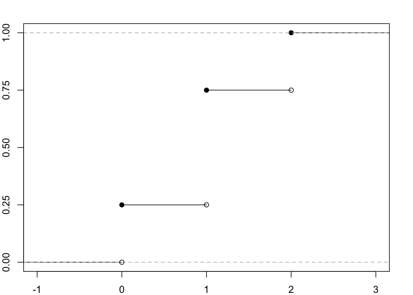
Figure 7.1: The CDF of the random variable X denoting the number of heads in two tosses of a symmetrical coin.
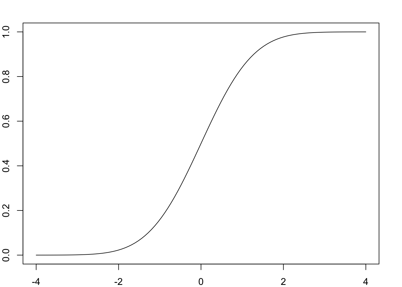
Figure 7.2: The CDF of a random variable Z having a standardised Gaussian distribution.
7.5 Transormations of random variables
7.5.1 Adding a constant to a random variable
If a constant \(a\) is added to random variable X, the expected value will shift accordingly, and the variance will not change:
\[\begin{equation} \mathbb{E}(X + a) = \mathbb{E}(X) + a \tag{7.15} \end{equation}\]
\[\begin{equation} \mathbb{V}(X + a) = \mathbb{V}(X) \tag{7.16} \end{equation}\]
7.5.2 Multiplying a random variable by a constant
If a random variable X is multiplied by the constant \(k\), then the expected value will be \(k\) times larger, the variance will be \(k^2\) times larger (the standard deviation will be \(k\) times larger).
\[\begin{equation} \mathbb{E}(k\cdot X)=k \cdot \mathbb{E}(X) \tag{7.17} \end{equation}\]
\[\begin{equation} \mathbb{V}(k \cdot X) = k^2 \cdot \mathbb{V}(X) \tag{7.18} \end{equation}\]
7.5.3 Adding random variables
If we have two random variables X and Y, the expected value of their sum (difference) will be equal to the sum (difference) of their expected values.
\[\begin{equation} \begin{matrix} \mathbb{E}(X + Y)=\mathbb{E}(X) + \mathbb{E}(Y) \\ \mathbb{E}(X - Y)=\mathbb{E}(X) - \mathbb{E}(Y) \\ \end{matrix} \:\:\:\: \text{ even when X and Y are dependent} \tag{7.19} \end{equation}\]
The variance of the sum of variables X and Y is equal to the sum of their variances, only when X and Y are independent. The variance of the difference of variables X and Y is equal to the sum (not: difference) of their variances.
\[\begin{equation} \begin{matrix} \mathbb{V}(X + Y) = \mathbb{V}(X) + \mathbb{V}(Y) \\ \mathbb{V}(X - Y) = \mathbb{V}(X)\: \mathbf{+}\: \mathbb{V}(Y) \\ \end{matrix} \:\:\:\: \text{ only when X and Y are independent} \tag{7.20} \end{equation}\]
A special case for which we apply the above formulae, taking into account a larger number of variables, is the sum of independent variables with identical distribution (i.i.d. - independent and identically distributed random variables).
If we have \(n\) such (i.i.d.) variables with mean \(\mu\) and standard deviation \(\sigma\) each, then their sum \(Y = X_1 + X_2 + .... + X_n\) has mean \(\mathbb{E}(Y) = \mathbb{E}(X_1) + \mathbb{E}(X_2) + .... + \mathbb{E}(X_n) = n\mu\), the variance \(\mathbb{V}(Y)=n\sigma^2\), and the standard deviation \(\sigma_Y = \sigma \sqrt{n}\).
7.6 Templates
Spreadsheets
Discrete random variable – calculator — Google spreadsheet
Discrete random variable – calculator — Excel template
R code
# Discrete probability distribution of a single variable
x <- c(0, 1, 4)
Px <- c(1/3, 1/3, 1/3)

# Check
if(length(x)!=length(Px))
{print("Both vectors should be of the same length.")}
if(!sum(Px)==1)
{print("The probabilities should add up to 1. ")}
if(any(Px<0))
{print("The probabilities cannot be negative. ")}

# Calculations
EX <- sum(x*Px)
VarX <- sum((x-EX)^2*Px)
SDX <- sqrt(VarX)
SkX <- sum((x-EX)^3*Px)/SDX^3
KurtX <- sum((x-EX)^4*Px)/SDX^4 - 3

print(c('Expected value' = EX,
        'Variance' = VarX,
        'Standard deviation' = SDX,
        'Skewness' = SkX,
        'Excess kurtosis' = KurtX))
## Expected value Variance Standard deviation Skewness Excess kurtosis
## 1.666667 2.888889 1.699673 0.528005 -1.500000# Joint probability distribution of two discrete random variables
x <- c(2, -1, -1)
y <- c(-1, 1, -1)
Pxy <- c(1/2, 1/3, 1-1/2-1/3) #sum(c(1/2, 1/3, 1/6))==1 may return FALSE for numerical reason
# Check
if(length(x)!=length(y) || length(x)!=length(Pxy))
{print("The vectors should be of the same length. ")}
if(!sum(Pxy)==1)
{print("The probabilities should add up to 1. ")}
if(any(Pxy<0))
{print("The probabilities cannot be negative. ")}
EX <- sum(x*Pxy)
VarX <- sum((x-EX)^2*Pxy)
SDX <- sqrt(VarX)
SkX <- sum((x-EX)^3*Pxy)/SDX^3
KurtX <- sum((x-EX)^4*Pxy)/SDX^4 - 3
EY <- sum(y*Pxy)
VarY <- sum((y-EY)^2*Pxy)
SDY <- sqrt(VarY)
SkY <- sum((y-EY)^3*Pxy)/SDY^3
KurtY <- sum((y-EY)^4*Pxy)/SDY^4 - 3
CovXY <- sum((x-EX)*(y-EY)*Pxy)
CorXY <- CovXY/(SDX*SDY)
print(c('Expected value of X' = EX,
'Variance of X' = VarX,
'Standard deviation of X' = SDX,
'Skewness of X' = SkX,
'Excess kurtosis of X' = KurtX,
'Expected value of Y' = EY,
'Variance of Y' = VarY,
'Standard deviation of Y' = SDY,
'Skewness of Y' = SkY,
'Excess kurtosis of Y' = KurtY,
'Covariance of X and Y' = CovXY,
'Correlation of X and Y' = CorXY
))## Expected value of X Variance of X Standard deviation of X Skewness of X Excess kurtosis of X
## 5.000000e-01 2.250000e+00 1.500000e+00 -3.289550e-17 -2.000000e+00
## Expected value of Y Variance of Y Standard deviation of Y Skewness of Y Excess kurtosis of Y
## -3.333333e-01 8.888889e-01 9.428090e-01 7.071068e-01 -1.500000e+00
## Covariance of X and Y Correlation of X and Y
## -1.000000e+00 -7.071068e-01Python code
# Discrete probability distribution of a single variable
x = [0, 1, 4]
Px = [1/3, 1/3, 1/3]

# Check
if len(x) != len(Px):
    print("Both vectors should be of the same length.")
if sum(Px) != 1:
    print("The probabilities should add up to 1. ")
if any(p < 0 for p in Px):
    print("The probabilities cannot be negative.")

# Calculations
EX = sum([a*b for a, b in zip(x, Px)])
VarX = sum([(a-EX)**2*b for a, b in zip(x, Px)])
SDX = VarX**0.5
SkX = sum([(a-EX)**3*b for a, b in zip(x, Px)]) / SDX**3
KurtX = sum([(a-EX)**4*b for a, b in zip(x, Px)]) / SDX**4 - 3

# Results
print({'Expected value': EX,
       'Variance': VarX,
       'Standard deviation': SDX,
       'Skewness': SkX,
       'Excess kurtosis': KurtX})
## {'Expected value': 1.6666666666666665, 'Variance': 2.888888888888889, 'Standard deviation': 1.699673171197595, 'Skewness': 0.5280049792181879, 'Excess kurtosis': -1.5000000000000002}# Joint probability distribution of two discrete random variables
x = [2, -1, -1]
y = [-1, 1, -1]
Pxy = [1/2, 1/3, 1-1/2-1/3]
# Check
if len(x) != len(y) or len(x) != len(Pxy):
print("The vectors should be of the same length. ")
if sum(Pxy) != 1:
print("The probabilities should add up to 1. ")
if any(p < 0 for p in Pxy):
print("The probabilities cannot be negative. ")
# Calculations
EX = sum([a*b for a, b in zip(x, Pxy)])
VarX = sum([(a-EX)**2*b for a, b in zip(x, Pxy)])
SDX = VarX**0.5
SkX = sum([(a-EX)**3*b for a, b in zip(x, Pxy)]) / SDX**3
KurtX = sum([(a-EX)**4*b for a, b in zip(x, Pxy)]) / SDX**4 - 3
EY = sum([a*b for a, b in zip(y, Pxy)])
VarY = sum([(a-EY)**2*b for a, b in zip(y, Pxy)])
SDY = VarY**0.5
SkY = sum([(a-EY)**3*b for a, b in zip(y, Pxy)]) / SDY**3
KurtY = sum([(a-EY)**4*b for a, b in zip(y, Pxy)]) / SDY**4 - 3
CovXY = sum([(a-EX)*(b-EY)*c for a, b, c in zip(x, y, Pxy)])
CorXY = CovXY / (SDX*SDY)
# Results
print({'Expected value of X': EX,
'Variance of X': VarX,
'Standard deviation of X': SDX,
'Skewness X': SkX,
'Excess kurtosis of X': KurtX,
'Expected value of Y': EY,
'Variance of Y': VarY,
'Standard deviation of Y': SDY,
'Skewness of Y': SkY,
'Excess kurtosis of Y': KurtY,
'Covariance of X and Y': CovXY,
'Correlation of X and Y': CorXY
})## {'Expected value of X': 0.5, 'Variance of X': 2.25, 'Standard deviation of X': 1.5, 'Skewness X': -3.289549702593056e-17, 'Excess kurtosis of X': -2.0, 'Expected value of Y': -0.33333333333333337, 'Variance of Y': 0.888888888888889, 'Standard deviation of Y': 0.9428090415820634, 'Skewness of Y': 0.7071067811865478, 'Excess kurtosis of Y': -1.4999999999999991, 'Covariance of X and Y': -0.9999999999999998, 'Correlation of X and Y': -0.7071067811865475}7.7 Exercises
Exercise 7.1 We toss four fair coins.
List all equally probable elementary events in the sample space. How many are there?
Let X be the number of heads. Assign values of the random variable X to each event.
Write down the probability distribution of the variable X in the form of a table.
Calculate the expected value of X.
Calculate the variance and standard deviation of X.
Exercise 7.2 A random variable has the following discrete probability distribution:
| \(x\) | \(\textbf{p}(x)\) |
|---|---|
| 10 | 0.2 |
| 11 | 0.3 |
| 12 | 0.2 |
| 13 | 0.1 |
| 14 | 0.2 |
Since the values taken by X are mutually exclusive events, the event \({ X ≤ 12 }\) is the sum of three mutually exclusive events:
\[\{ X = 10 \} \cup \{ X = 11 \} \cup \{ X = 12 \}\]
Find:
- \(\mathbb{P}(X ≤ 12)\)
- \(\mathbb{P}(X > 12)\)
- \(\mathbb{P}(X ≤ 14)\)
- \(\mathbb{P}(X = 14)\)
- \(\mathbb{P}(X ≤ 11\:\text{or}\:X > 12)\)
Exercise 7.3 A car dealer records the number of vehicles sold each day. The data is used to determine the following probability distribution of daily sales:
| \(x\) | \(\textbf{p}(x)\) |
|---|---|
| 0 | 0.1 |
| 1 | 0.1 |
| 2 | 0.2 |
| 3 | 0.2 |
| 4 | 0.3 |
| 5 | 0.1 |
What is the probability that the number of cars sold tomorrow will be between 2 and 4 (both inclusive)?
Find the CDF of the number of cars sold daily.
Exercise 7.4 In a certain gambling game, a participant draws one card from a regular deck (52 cards). If the card drawn is a queen or jack, the participant is paid 30 PLN, if a king or ace – the win is 8 PLN. In the case of another card, the person pays 5 PLN. What is the expected cash flow? What is the standard deviation of the cash flow?
Exercise 7.5 We roll a perfectly balanced die once. Let Y denote the number of dots obtained. What is the expected value and variance of Y?
Exercise 7.6 A certain basketball player, making a three-point shot, hits the basket with a probability of 0.2. Suppose that the success rates in two consecutive throws are independent of each other, i.e. scoring or not in the first throw does not change the probability in the second throw. Let the random variable X denote the number of hits in two throws. What are the mean and variance of the variable X?
Exercise 7.7 The following probability distribution is given:
| \(x\) | \(\textbf{p}(x)\) |
|---|---|
| 1 | 0.2 |
| 2 | 0.4 |
| 5 | 0.3 |
| 10 | 0.1 |
Find \(\mathbb{E}(X)\).
Find \(sigma^2 = \mathbb{E}[ (X-\mu)^2]\).
How much is \(\sigma\)?
Will this random variable ever take on the value of \(\sigma\)? How do you interpret the expected value?
Give an example of a random variable that can take on a value equal to its expected value.
Exercise 7.8 What is the expected value and standard deviation of the Bernoulli distribution with parameter \(p\)?
| \(x\) | \(\textbf{p}(x)\) |
|---|---|
| 1 | \(p\) |
| 0 | \((1-p)\) |
Exercise 7.9 What is the expected profit (or loss) in the Polish Lotto with the following assumptions: one bet costs 3 zlotys, for a three you get 24 zlotys, for a four you get 200 zlotys on average, for a five you get 5000 zlotys, and for a six you get 9 million zlotys?
How much would we have to receive, as a minimum, for a sixth for the expected profit to be positive?
Exercise 7.10 A stanine scale (the name comes from ‘standardised nine’) is created when we transform a variable (e.g. exam results or total scores in a psychometric test) as follows: 4% of the lowest scores go to category (‘stanine’) 1, another 7% to category 2, 12% to category 3, 17% to category 4, 20% of the middle scores to category 5, another 17% to category 6, 12% to 7, 7% to 8 and 4% of the highest scores to category 9. Treat the stanines as a new variable taking integer values from 1 to 9. Calculate what the mean and standard deviation of the new variable.
Exercise 7.11 Similar to the stanine scale is the sten system (from ‘standardised ten’): 2.27% of the lowest scores go to grade 1, 4.41% to grade 2, 9.18% to grade 3, 14.99% to grade 4, 19.15% to grade 5. Similarly, above the median 19.15% of the scores go to grade 6, 14.99% to grade 7, 9.18% to grade 8, 4.41% to grade 9, while 2.27% of the highest scores go to grade 10. Calculate the mean and standard deviation of the sten scale.
Exercise 7.12 Calculate the expected value of a bet if in the American roulette we bet on:
- Straight Up (a single number)
- Split (two numbers)
Street (three numbers)
Corner (four numbers)
Top Line (Five)
Six Line / Double Street
Column
Dozen (1 - 12, 13 - 24, or 25 - 36)
Even, or Odd
Red, or Black
1st 18, or 2nd 18