C Templates
Notes
Google spreadsheets are, of course, read-only. To use the templates, you need to log in to your Google account and then select File > Make a copy from the menu.
In the sheets, I tried to maintain the following color convention:
Green indicates areas that need to be changed (e.g., data entry).
Yellow highlights the most important results, formulas in these cells (and other non-green cells) should not be changed or overwritten.
Some cells may contain calculations even though they appear empty. Be cautious and avoid overwriting these cells.
Excel templates may not work in Excel 2007 due to the limited availability of statistical functions in this version. Excel 2007 users are encouraged to report which sheets do not work – maybe we will be able to find a workaround .
The templates are continuously being developed, so any comments, suggestions, or error reports are welcome.
C.1 Bayes' formula
Bayes' formula — Google spreadsheet
Bayes' formula — Excel template
# Hypotheses: descriptions (optional)
hypotheses <- c("Disease", "No disease")

# Prior
prior <- c(.001, .999)

# Likelihood
likelihood <- c(.95, .01)

# Posterior
posterior <- prior*likelihood
posterior <- posterior/sum(posterior)

# Check
if(length(prior)!=length(likelihood))
{print("Both vectors (prior and likelihood) should be the same length. ")}
if(sum(prior)!=1){
  print("Suma prawdopodobieństw w rozkładzie zaczątkowym (prior) powinna być równa 1.")}
if (!exists("hypotheses") || length(hypotheses)!=length(prior)) {
  hipotezy <- paste0('H', 1:length(prior))
}

# Wynik w formie ramki danych:
print(data.frame(
  Hypothesis = hypotheses, `Prior` = prior, `Likelihood` = likelihood, `Posterior` = posterior
))
## Hypothesis Prior Likelihood Posterior
## 1 Disease 0.001 0.95 0.08683729
## 2 No disease 0.999 0.01 0.91316271# Chart
library(ggplot2)
hypotheses<-factor(hypotheses, levels=hypotheses)
df <- data.frame(Hypotheses = c(hypotheses, hypotheses),
`Distribution` = factor(c(rep("prior", length(prior)), rep("posterior", length(posterior))),
levels=c("prior", "posterior")
),
`Probability` = c(prior, posterior)
)
ggplot(data=df, aes(x=Hypotheses, y=`Probability`, fill=`Distribution`)) +
geom_bar(stat="identity", position=position_dodge())+
geom_text(aes(label = format(round(`Probability`,4), nsmall=4), group=`Distribution`),
position = position_dodge(width = .9), vjust = -0.2)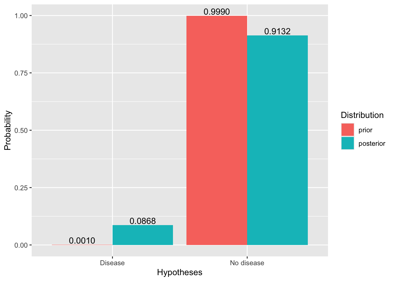
# Hypotheses: descriptions (optional)
hypotheses = ["Disease", "No disease"]

# Prior
prior = [.001, .999]

# Likelihood
likelihood = [.95, .01]

# Posterior
posterior = [a*b for a, b in zip(prior, likelihood)]
posterior = [p/sum(posterior) for p in posterior]

# Check
if len(prior) != len(likelihood):
    print("Both vectors (prior and likelihood) should be the same length. ")
if sum(prior) != 1:
    print("The sum of probabilities in the prior distribtuion should be 1.")
if not "hypotheses" in locals() or len(hypotheses) != len(prior):
    hypotheses = ["H" + str(i) for i in range(1, len(prior)+1)]

# Wynik w formie ramki danych:
import pandas as pd
df = pd.DataFrame({
    "Hypothesis": hypotheses,
    "Prior": prior,
    "Likelihood": likelihood,
    "Posterior": posterior
})
print(df)
## Hypothesis Prior Likelihood Posterior
## 0 Disease 0.001 0.95 0.086837
## 1 No disease 0.999 0.01 0.913163import numpy as np
import matplotlib.pyplot as plt
x = np.arange(len(hypotheses))
width = 0.375
fig, ax = plt.subplots(layout='constrained')
rects = ax.bar(x-width/2, np.round(prior, 4), width, label = 'zaczątek')
ax.bar_label(rects, padding=3)
rects = ax.bar(x+width/2, np.round(posterior, 4), width, label = 'posterior')
ax.bar_label(rects, padding=3)
ax.set_ylabel('probability')
ax.set_xlabel('hypotheses')
ax.set_xticks(x, hypotheses)
ax.legend(loc='upper left', ncols=2)
#ax.set_ylim(0, np.max([prior, posterior])*1.2)
plt.show()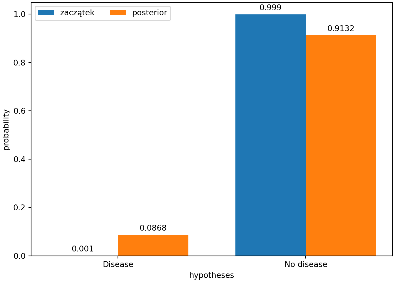
C.2 Distributions
C.2.1 Discrete random variable
Discrete random variable – calculator — Google spreadsheet
Discrete random variable – calculator — Excel template
# Discrete probability distribution of a single variable
x <- c(0, 1, 4)
Px <- c(1/3, 1/3, 1/3)

# Check
if(length(x)!=length(Px))
{print("Both vectors should be of the same length.")}
if(!sum(Px)==1)
{print("The probabilities should add up to 1. ")}
if(any(Px<0))
{print("The probabilities cannot be negative. ")}

# Calculations
EX <- sum(x*Px)
VarX <- sum((x-EX)^2*Px)
SDX <- sqrt(VarX)
SkX <- sum((x-EX)^3*Px)/SDX^3
KurtX <- sum((x-EX)^4*Px)/SDX^4 - 3

print(c('Expected value' = EX,
        'Variance' = VarX,
        'Standard deviation' = SDX,
        'Skewness' = SkX,
        'Excess kurtosis' = KurtX))
## Expected value Variance Standard deviation Skewness Excess kurtosis
## 1.666667 2.888889 1.699673 0.528005 -1.500000# Joint probability distribution of two discrete random variables
x <- c(2, -1, -1)
y <- c(-1, 1, -1)
Pxy <- c(1/2, 1/3, 1-1/2-1/3) #sum(c(1/2, 1/3, 1/6))==1 may return FALSE for numerical reason
# Check
if(length(x)!=length(y) || length(x)!=length(Pxy))
{print("The vectors should be of the same length. ")}
if(!sum(Pxy)==1)
{print("The probabilities should add up to 1. ")}
if(any(Pxy<0))
{print("The probabilities cannot be negative. ")}
EX <- sum(x*Pxy)
VarX <- sum((x-EX)^2*Pxy)
SDX <- sqrt(VarX)
SkX <- sum((x-EX)^3*Pxy)/SDX^3
KurtX <- sum((x-EX)^4*Pxy)/SDX^4 - 3
EY <- sum(y*Pxy)
VarY <- sum((y-EY)^2*Pxy)
SDY <- sqrt(VarY)
SkY <- sum((y-EY)^3*Pxy)/SDY^3
KurtY <- sum((y-EY)^4*Pxy)/SDY^4 - 3
CovXY <- sum((x-EX)*(y-EY)*Pxy)
CorXY <- CovXY/(SDX*SDY)
print(c('Expected value of X' = EX,
'Variance of X' = VarX,
'Standard deviation of X' = SDX,
'Skewness of X' = SkX,
'Excess kurtosis of X' = KurtX,
'Expected value of Y' = EY,
'Variance of Y' = VarY,
'Standard deviation of Y' = SDY,
'Skewness of Y' = SkY,
'Excess kurtosis of Y' = KurtY,
'Covariance of X and Y' = CovXY,
'Correlation of X and Y' = CorXY
))## Expected value of X Variance of X Standard deviation of X Skewness of X Excess kurtosis of X
## 5.000000e-01 2.250000e+00 1.500000e+00 -3.289550e-17 -2.000000e+00
## Expected value of Y Variance of Y Standard deviation of Y Skewness of Y Excess kurtosis of Y
## -3.333333e-01 8.888889e-01 9.428090e-01 7.071068e-01 -1.500000e+00
## Covariance of X and Y Correlation of X and Y
## -1.000000e+00 -7.071068e-01# Discrete probability distribution of a single variable
x = [0, 1, 4]
Px = [1/3, 1/3, 1/3]
# Check
if len(x) != len(Px):
print("Both vectors should be of the same length.")
if sum(Px) != 1:
print("The probabilities should add up to 1. ")
if any(p < 0 for p in Px):
print("The probabilities cannot be negative.")
# Calculations
EX = sum([a*b for a, b in zip(x, Px)])
VarX = sum([(a-EX)**2*b for a, b in zip(x, Px)])
SDX = VarX**0.5
SkX = sum([(a-EX)**3*b for a, b in zip(x, Px)]) / SDX**3
KurtX = sum([(a-EX)**4*b for a, b in zip(x, Px)]) / SDX**4 - 3
# Results
print({'Expected value': EX,
'Variance': VarX,
'Standard deviation': SDX,
'Skewness': SkX,
'Excess kurtosis': KurtX})## {'Expected value': 1.6666666666666665, 'Variance': 2.888888888888889, 'Standard deviation': 1.699673171197595, 'Skewness': 0.5280049792181879, 'Excess kurtosis': -1.5000000000000002}# Joint probability distribution of two discrete random variables
x = [2, -1, -1]
y = [-1, 1, -1]
Pxy = [1/2, 1/3, 1-1/2-1/3]
# Check
if len(x) != len(y) or len(x) != len(Pxy):
print("The vectors should be of the same length. ")
if sum(Pxy) != 1:
print("The probabilities should add up to 1. ")
if any(p < 0 for p in Pxy):
print("The probabilities cannot be negative. ")
# Calculations
EX = sum([a*b for a, b in zip(x, Pxy)])
VarX = sum([(a-EX)**2*b for a, b in zip(x, Pxy)])
SDX = VarX**0.5
SkX = sum([(a-EX)**3*b for a, b in zip(x, Pxy)]) / SDX**3
KurtX = sum([(a-EX)**4*b for a, b in zip(x, Pxy)]) / SDX**4 - 3
EY = sum([a*b for a, b in zip(y, Pxy)])
VarY = sum([(a-EY)**2*b for a, b in zip(y, Pxy)])
SDY = VarY**0.5
SkY = sum([(a-EY)**3*b for a, b in zip(y, Pxy)]) / SDY**3
KurtY = sum([(a-EY)**4*b for a, b in zip(y, Pxy)]) / SDY**4 - 3
CovXY = sum([(a-EX)*(b-EY)*c for a, b, c in zip(x, y, Pxy)])
CorXY = CovXY / (SDX*SDY)
# Results
print({'Expected value of X': EX,
'Variance of X': VarX,
'Standard deviation of X': SDX,
'Skewness X': SkX,
'Excess kurtosis of X': KurtX,
'Expected value of Y': EY,
'Variance of Y': VarY,
'Standard deviation of Y': SDY,
'Skewness of Y': SkY,
'Excess kurtosis of Y': KurtY,
'Covariance of X and Y': CovXY,
'Correlation of X and Y': CorXY
})## {'Expected value of X': 0.5, 'Variance of X': 2.25, 'Standard deviation of X': 1.5, 'Skewness X': -3.289549702593056e-17, 'Excess kurtosis of X': -2.0, 'Expected value of Y': -0.33333333333333337, 'Variance of Y': 0.888888888888889, 'Standard deviation of Y': 0.9428090415820634, 'Skewness of Y': 0.7071067811865478, 'Excess kurtosis of Y': -1.4999999999999991, 'Covariance of X and Y': -0.9999999999999998, 'Correlation of X and Y': -0.7071067811865475}C.2.2 Parametric discrete distributions
Discrete distributions calculator — Google spreadsheet
Discrete distributions calculator — Excel template
# Binomial distribution
n <- 18
p <- 0.6
from <- 12
to <- 14

result <- pbinom(to, n, p)-pbinom(from-1, n, p)
if (from > to) {
  # error from > to
  print("!!! 'From' cannot be greater than 'to' !!!")
} else {
  p=paste0("P(", from, " <= X <= ", to, ")")
  print(p)
  print(result)
}
## [1] "P(12 <= X <= 14)"
## [1] 0.3414956# Poisson
lambda <- 5/3
from <- 2
to <- Inf
result <- ppois(to, lambda)-ppois(from-1, lambda)
if (from > to) {
# error from > to
print("!!! 'From' cannot be greater than 'to' !!!")
} else {
p=paste0("P(", from, " <= X <= ", to, ")")
print(p)
print(result)
}## [1] "P(2 <= X <= Inf)"
## [1] 0.4963317# Hypergeometric distribution
N <- 49
r <- 6
n <- 6
from <- 3
to <- 6
result <- phyper(to, r, N-r, n)-phyper(from-1, r, N-r, n)
if (from > to) {
# error from > to
print("!!! 'From' cannot be greater than 'to' !!!")
} else {
p=paste0("P(", from, " <= X <= ", to, ")")
print(p)
print(result)
}## [1] "P(3 <= X <= 6)"
## [1] 0.01863755from scipy.stats import binom, poisson, hypergeom
# Binomial distribution
n = 18
p = 0.6
_from = 12
_to = 14
result = binom.cdf(_to, n, p) - binom.cdf(_from-1, n, p)
if _from > _to:
print("!!! 'From' cannot be greater than 'to' !!!")
else:
p = "P(" + str(_from) + " <= X <= " + str(_to) + ")"
print(p)
print(result)## P(12 <= X <= 14)
## 0.34149556326865305
# Poisson distribution
lambda_val = 5/3
from_val = 2
to_val = float('inf')

result = poisson.cdf(to_val, lambda_val) - poisson.cdf(from_val-1, lambda_val)

if from_val > to_val:
    print("!!! 'From' cannot be greater than 'to' !!!")
else:
    p = "P(" + str(from_val) + " <= X <= " + str(to_val) + ")"
    print(p)
    print(result)
## P(2 <= X <= inf)
## 0.49633172576650164
# Hypergeometric distribution
N = 49
r = 6
n = 6
_from = 3
_to = 6

result = hypergeom.cdf(_to, N, r, n) - hypergeom.cdf(_from-1, N, r, n)

if _from > _to:
    print("!!! 'From' cannot be greater than 'to' !!!")
else:
    p = "P(" + str(_from) + " <= X <= " + str(_to) + ")"
    print(p)
    print(result)
## P(3 <= X <= 6)
## 0.018637545002022304C.2.3 Continuous distributions
Normal distribution calculator — Google spreadsheet
Normal distribution calculator — Excel template
##### 1. Area under PDF #####
# Gaussian distribution parameters:
# mean:
m <- 0
# standard deviation:
sd <- 2

# Calculating the area under PDF
# from
# *for minus infinity use from <- -Inf
from <- -Inf
# to
# *for plus infinity use to <- Inf
to <- 2

# Data validation, calculation
if (from > to) {
  # from > to error
  print("!!! _From_ cannot be greater than _to_ !!!")
} else {

  # Probability notation

  if (to==Inf) {
    p=paste0("P(X>", from, ")")
  } else if (from==-Inf) {
    p=paste0("P(X<", to, ")")
  } else {
    p=paste0("P(", from, "<X<", to, ")")
  }
  print(p)

  # Calculating the area for the given segment:
  result<-pnorm(to, m, sd)-pnorm(from, m, sd)
  print(result)
}
## [1] "P(X<2)"
## [1] 0.8413447# Plot
library(ggplot2)
x1=if(from==-Inf){min(-4*sd+m, to-2*sd)} else {min(from-2*sd, -4*sd+m)}
x2=if(to==Inf){max(4*sd+m, from+2*sd)} else {max(to+2*sd, 4*sd+m)}
df<-data.frame(y=c(0, 0),
x=c(if(from==-Inf){NA}else{from}, if(to==-Inf){NA}else{to}),
label=c(if(from==-Inf){NA}else{from}, if(to==-Inf){NA}else{to}))
plt<-ggplot(NULL, aes(c(x1, x2))) +
theme_minimal() +
xlab('') +
ylab('') +
geom_area(stat = "function",
fun = function(x){dnorm(x, m, sd)},
fill = "orange",
xlim = c(if(from==-Inf){x1}else{from}, if(to==Inf){x2}else{to})) +
geom_line(stat = "function", fun = function(x){dnorm(x, m, sd)}, col = "blue", lty=2, lwd=1) +
scale_x_continuous(breaks=c(m, m-sd, m-2*sd, m+sd, m+2*sd, m-3*sd, m+3*sd, m-4*sd, m+4*sd)) +
geom_point(data = df, aes(x=x, y=y), shape=4) +
geom_text(data = df, aes(x=x, y=y, label=signif(label, 6)), vjust=1.4) +
annotate("text", label = paste0("M = ", m, "\nSD = ", sd, "\n", p, " = ", signif(result,6)),
x = x1, y = dnorm(m, m, sd)*1.2, size = 6, hjust="inward", vjust = "inward")
suppressWarnings(print(plt))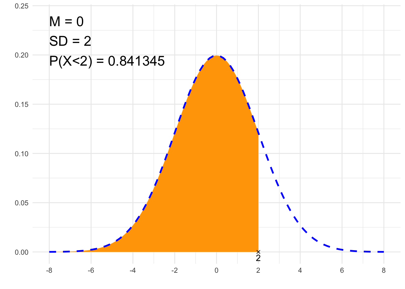
##### 2. Find x #####
# Gaussian distribution parameters:
# mean:
m <- 1
# standard deviation:
sd <- 3

# The area under PDF:
P <- 0.95

# 'L' - left, 'R' - right, 'S' - symmetrical (middle)
typ <- 'L'

# Calculations
from <- -qnorm(if(typ=='L'){1} else if(typ=='R'){P} else {1-(1-P)/2})*sd+m
to <- qnorm(if(typ=='L'){P} else if(typ=='R'){1} else {1-(1-P)/2})*sd+m

# P notation
if (to==Inf) {
  p=paste0("P(X>", signif(from, 6), ")")
} else if (from==-Inf) {
  p=paste0("P(X<", signif(to, 6), ")")
} else {
  p=paste0("P(", signif(from, 6), " < X < ", signif(to, 6), ")")
}
print(paste0(p, " = ", P))
## [1] "P(X<5.93456) = 0.95"# Plot
library(ggplot2)
x1=if(from==-Inf){min(-4*sd+m, to-2*sd)} else {min(from-2*sd, -4*sd+m)}
x2=if(to==Inf){max(4*sd+m, from+2*sd)} else {max(to+2*sd, 4*sd+m)}
df<-data.frame(y=c(0, 0),
x=c(if(from==-Inf){NA}else{from}, if(to==-Inf){NA}else{to}),
label=c(if(from==-Inf){NA}else{from}, if(to==-Inf){NA}else{to}))
plt<-ggplot(NULL, aes(c(x1, x2))) +
theme_minimal() +
xlab('') +
ylab('') +
geom_area(stat = "function",
fun = function(x){dnorm(x, m, sd)},
fill = "orange",
xlim = c(if(from==-Inf){x1}else{from}, if(to==Inf){x2}else{to})) +
geom_line(stat = "function", fun = function(x){dnorm(x, m, sd)}, col = "blue", lty=2, lwd=1) +
scale_x_continuous(breaks=c(m, m-sd, m-2*sd, m+sd, m+2*sd, m-3*sd, m+3*sd, m-4*sd, m+4*sd)) +
geom_point(data = df, aes(x=x, y=y), shape=4) +
geom_text(data = df, aes(x=x, y=y, label=signif(label, 6)), vjust=1.4) +
annotate("text", label = paste0("M = ", m, "\nSD = ", sd, "\n", p, " = ", P),
x = x1, y = dnorm(m, m, sd)*1.2, size = 6, hjust="inward", vjust = "inward")
suppressWarnings(print(plt))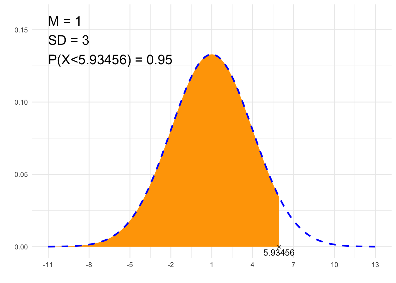
from scipy.stats import norm
##### 1. Area under PDF #####
# Gaussian distribution parameters:
# mean:
m = 0
# standard deviation:
sd = 2
# Calculating the area under PDF
# from
# *for minus infinity use _from = float('-inf')
_from = float('-inf')
# to
_to = 2

# Data validation, calculation
if _from > _to:
    print("!!! _From_ cannot be greater than _to_ !!!")
else:
    if _to == float('inf'):
        p = "P(X>" + str(_from) + ")"
    elif _from == float('-inf'):
        p = "P(X<" + str(_to) + ")"
    else:
        p = "P(" + str(_from) + "<X<" + str(_to) + ")"
    print(p)

    result = norm.cdf(_to, m, sd) - norm.cdf(_from, m, sd)
    print(result)
## P(X<2)
## 0.8413447460685429##### 2. Find x #####
import numpy as np
from scipy.stats import norm
# Gaussian distribution parameters:
# mean:
m = 1
# standard deviation:
sd = 3
# The area under PDF:
P = 0.95
# 'L' - left, 'R' - right, 'S' - symmetrical (middle)
typ = 'L'
# Obliczenia
if typ == 'L':
_from = -norm.ppf(1) * sd + m
_to = norm.ppf(P) * sd + m
elif typ == 'R':
_from = -norm.ppf(P) * sd + m
_to = norm.ppf(1) * sd + m
else:
_from = -norm.ppf(1-(1-P)/2) * sd + m
_to = norm.ppf(1-(1-P)/2) * sd + m
# Zapis prawdopodobieństwa
if np.isinf(_to):
p = f"P(X>{np.round(_from, 6)})"
elif np.isinf(_from):
p = f"P(X<{np.round(_to, 6)})"
else:
p = f"P({np.round(_from, 6)} < X < {np.round(_to, 6)})"
print(f"{p} = {P}")## P(X<5.934561) = 0.95Student-t distribution calculator — Google spreadsheet
Student-t distribution calculator — Excel template
##### 1. Area under PDF #####
# Parameter:
# Degrees of freedom:
nu <- 23

# Calculating the area under PDF
# from
# *for minus infinity use from <- -Inf
from <- 1
# to
# *for plus infinity use to <- Inf
to <- Inf

# Data validation, calculation
if (from > to) {
  # from > to error
  print("!!! _From_ cannot be greater than _to_ !!!")
} else {

  # Probability notation

  if (to==Inf) {
    p=paste0("P(X>", from, ")")
  } else if (from==-Inf) {
    p=paste0("P(X<", to, ")")
  } else {
    p=paste0("P(", from, "<X<", to, ")")
  }
  print(p)

  # Calculating the area for the given segment:
  result<-pt(to, nu)-pt(from, nu)
  print(result)
}
## [1] "P(X>1)"
## [1] 0.1638579# Plot
library(ggplot2)
x1=-5
x2=5
df<-data.frame(y=c(0, 0),
x=c(if(from==-Inf){NA}else{from}, if(to==-Inf){NA}else{to}),
label=c(if(from==-Inf){NA}else{from}, if(to==-Inf){NA}else{to}))
plt<-ggplot(NULL, aes(c(x1, x2))) +
theme_minimal() +
xlab('') +
ylab('') +
geom_area(stat = "function",
fun = function(x){dt(x, nu)},
fill = "orange",
xlim = c(if(from==-Inf){x1}else{from}, if(to==Inf){x2}else{to})) +
geom_line(stat = "function", fun = function(x){dt(x, nu)}, col = "blue", lty=2, lwd=1) +
geom_point(data = df, aes(x=x, y=y), shape=4) +
geom_text(data = df, aes(x=x, y=y, label=signif(label, 6)), vjust=1.4) +
annotate("text", label = paste0("ν = ", nu, "\n", p, " = ", signif(result,6)),
x = x1, y = dt(0, nu)*1.2, size = 6, hjust="inward", vjust = "inward")
suppressWarnings(print(plt))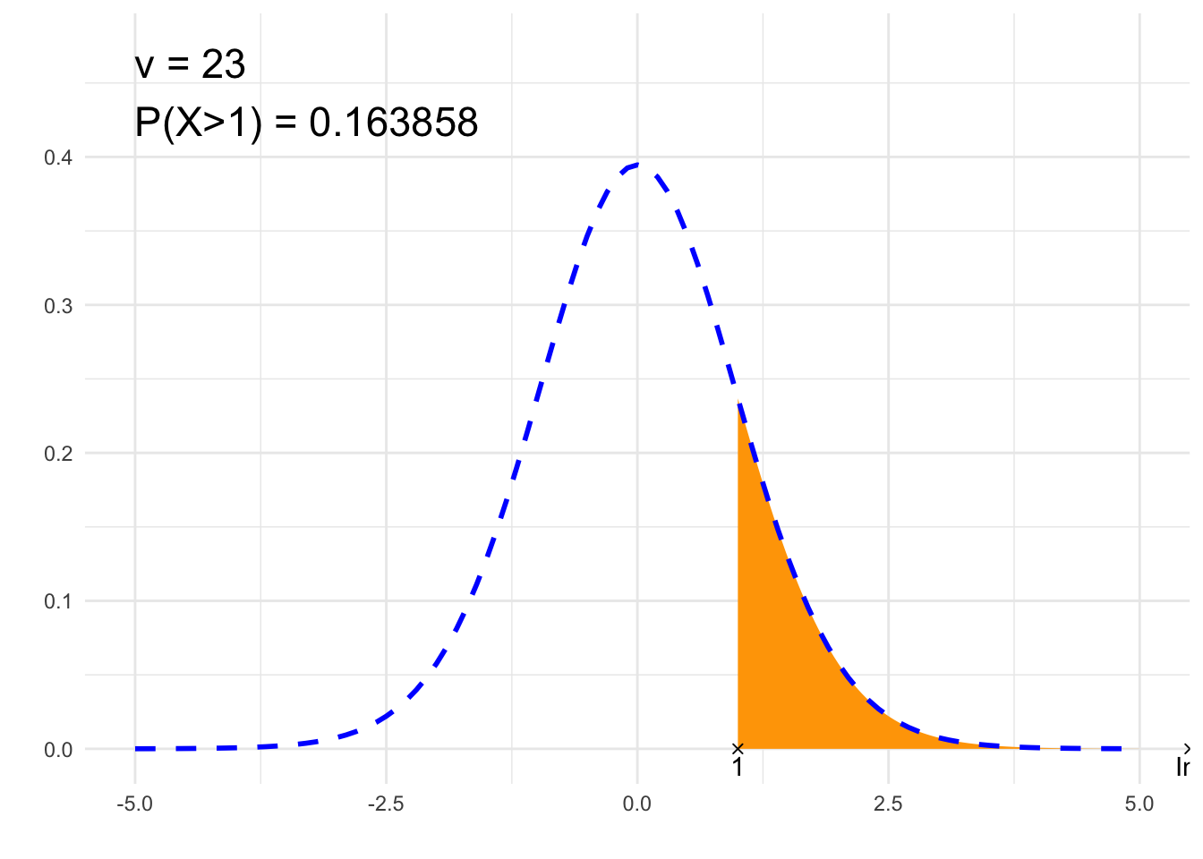
##### 2. Find x #####
# Parameter:
# Degrees of freedom:
nu <- 23

# The area under PDF:
P <- 0.95

# 'L' - left, 'R' - right, 'S' - symmetrical (middle)
typ <- 'S'

# Calculations
from <- -qt(if(typ=='L'){1} else if(typ=='R'){P} else {1-(1-P)/2}, nu)
to <- qt(if(typ=='L'){P} else if(typ=='R'){1} else {1-(1-P)/2}, nu)

# P notation
if (to==Inf) {
  p=paste0("P(X>", signif(from, 6), ")")
} else if (from==-Inf) {
  p=paste0("P(X<", signif(to, 6), ")")
} else {
  p=paste0("P(", signif(from, 6), " < X < ", signif(to, 6), ")")
}
print(paste0(p, " = ", P))
## [1] "P(-2.06866 < X < 2.06866) = 0.95"# Plot
library(ggplot2)
x1=-5
x2=5
df<-data.frame(y=c(0, 0),
x=c(if(from==-Inf){NA}else{from}, if(to==-Inf){NA}else{to}),
label=c(if(from==-Inf){NA}else{from}, if(to==-Inf){NA}else{to}))
plt<-ggplot(NULL, aes(c(x1, x2))) +
theme_minimal() +
xlab('') +
ylab('') +
geom_area(stat = "function",
fun = function(x){dt(x, nu)},
fill = "orange",
xlim = c(if(from==-Inf){x1}else{from}, if(to==Inf){x2}else{to})) +
geom_line(stat = "function", fun = function(x){dt(x, nu)}, col = "blue", lty=2, lwd=1) +
geom_point(data = df, aes(x=x, y=y), shape=4) +
geom_text(data = df, aes(x=x, y=y, label=signif(label, 6)), vjust=1.4) +
annotate("text", label = paste0("ν = ", nu, "\n", p, " = ", P),
x = x1, y = dt(0, nu)*1.2, size = 6, hjust="inward", vjust = "inward")
suppressWarnings(print(plt))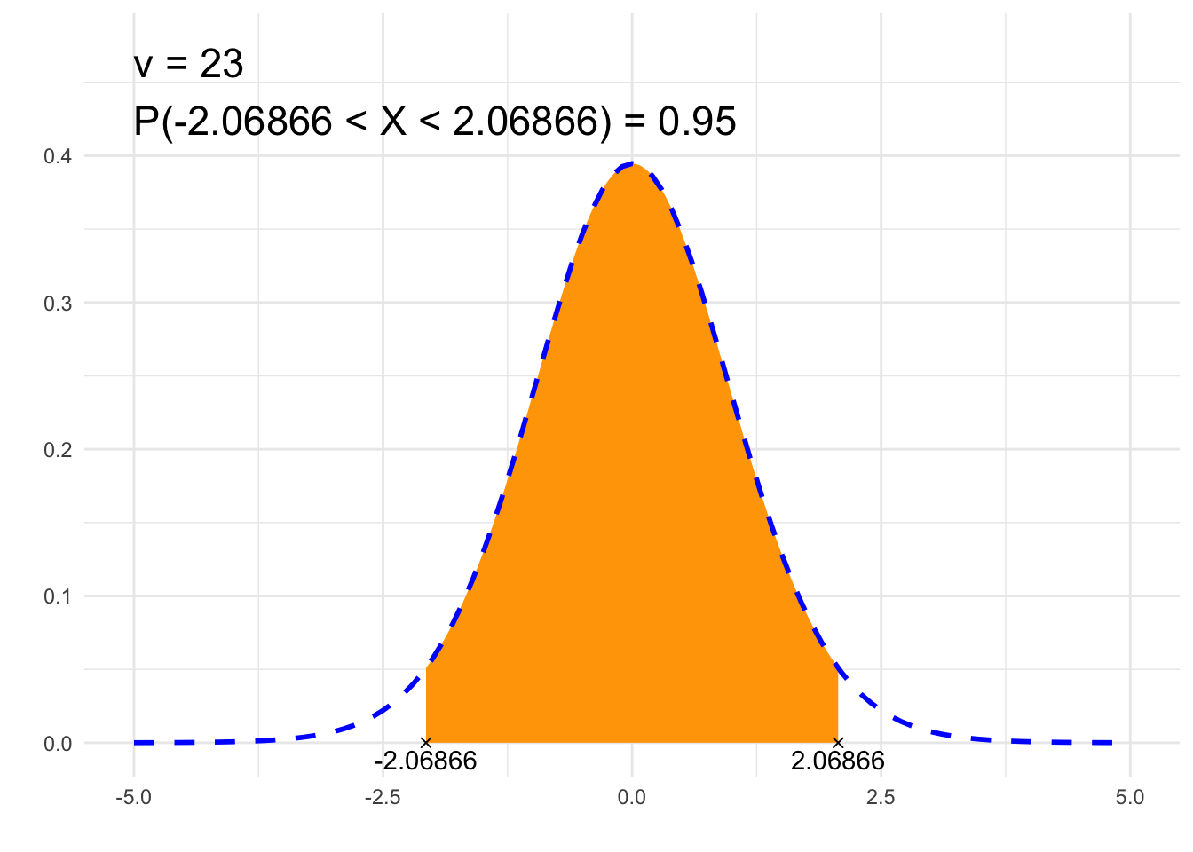
from scipy.stats import t
##### 1. Area under PDF #####
# Parameter:
# Degrees of freedom:
nu = 23

# Calculating the area under PDF
# from
# *for minus infinity use _from = float('-inf')
_from = 1
# to
# *for plus infinity use _to = float('inf')
_to = float('inf')

if _from > _to:
    print("!!! _From_ cannot be greater than _to_ !!!")
else:
    if _to == float('inf'):
        p = "P(X>" + str(_from) + ")"
    elif _from == float('-inf'):
        p = "P(X<" + str(_to) + ")"
    else:
        p = "P(" + str(_from) + "<X<" + str(_to) + ")"
    print(p)
    result = t.cdf(_to, nu) - t.cdf(_from, nu)
    print(result)
## P(X>1)
## 0.16385790307142933
##### 2. Find x #####

import numpy as np
from scipy.stats import t

# Parameter:
# Degrees of freedom:
nu = 23

# The area under PDF:
P = 0.95

# 'L' - left, 'R' - right, 'S' - symmetrical (middle)
typ = 'S'

# Obliczenia
if typ == 'L':
    _from = -t.ppf(1, nu)
    _to = t.ppf(P, nu)
elif typ == 'R':
    _from = -t.ppf(P, nu)
    _to = t.ppf(1)
else:
    _from = -t.ppf(1-(1-P)/2, nu)
    _to = t.ppf(1-(1-P)/2, nu)

# P notation
if np.isinf(_to):
    p = f"P(X>{np.round(_from, 6)})"
elif np.isinf(_from):
    p = f"P(X<{np.round(_to, 6)})"
else:
    p = f"P({np.round(_from, 6)} < X < {np.round(_to, 6)})"
print(f"{p} = {P}")
## P(-2.068658 < X < 2.068658) = 0.95Chi-square distribution calculator — Google spreadsheet
##### 1. Area under PDF #####
# Parameter:
# Degrees of freedom:
nu <- 4

# Calculating the area under PDF
# from
# *for minus infinity use from <- -Inf
from <- 10
# do
# *for plus infinity use to <- Inf
to <- Inf

# Data validation, calculation
if (from > to) {
  # from > to error
  print("!!! _From_ cannot be greater than _to_ !!!")
} else {

  # Probability notation

  if (to==Inf) {
    p=paste0("P(X>", from, ")")
  } else if (from==-Inf) {
    p=paste0("P(X<", to, ")")
  } else {
    p=paste0("P(", from, "<X<", to, ")")
  }
  print(p)

  # Calculating the area for the specified segment:
  result<-pchisq(to, nu)-pchisq(from, nu)
  print(result)
}
## [1] "P(X>10)"
## [1] 0.04042768# Plot
library(ggplot2)
x1=0
x2=nu*4
df<-data.frame(y=c(0, 0),
x=c(if(from==-Inf){NA}else{from}, if(to==-Inf){NA}else{to}),
label=c(if(from==-Inf){NA}else{from}, if(to==-Inf){NA}else{to}))
plt<-ggplot(NULL, aes(c(x1, x2))) +
theme_minimal() +
xlab('') +
ylab('') +
geom_area(stat = "function",
fun = function(x){dchisq(x, nu)},
fill = "orange",
xlim = c(if(from==-Inf){x1}else{from}, if(to==Inf){x2}else{to})) +
geom_line(stat = "function", fun = function(x){dchisq(x, nu)}, col = "blue", lty=2, lwd=1) +
geom_point(data = df, aes(x=x, y=y), shape=4) +
geom_text(data = df, aes(x=x, y=y, label=signif(label, 6)), vjust=1.4) +
annotate("text", label = paste0("ν = ", nu, "\n", p, " = ", signif(result,4)),
x = 4*nu, y = dchisq(max(nu-2,0), nu), size = 6, hjust="inward", vjust = "inward")
suppressWarnings(print(plt))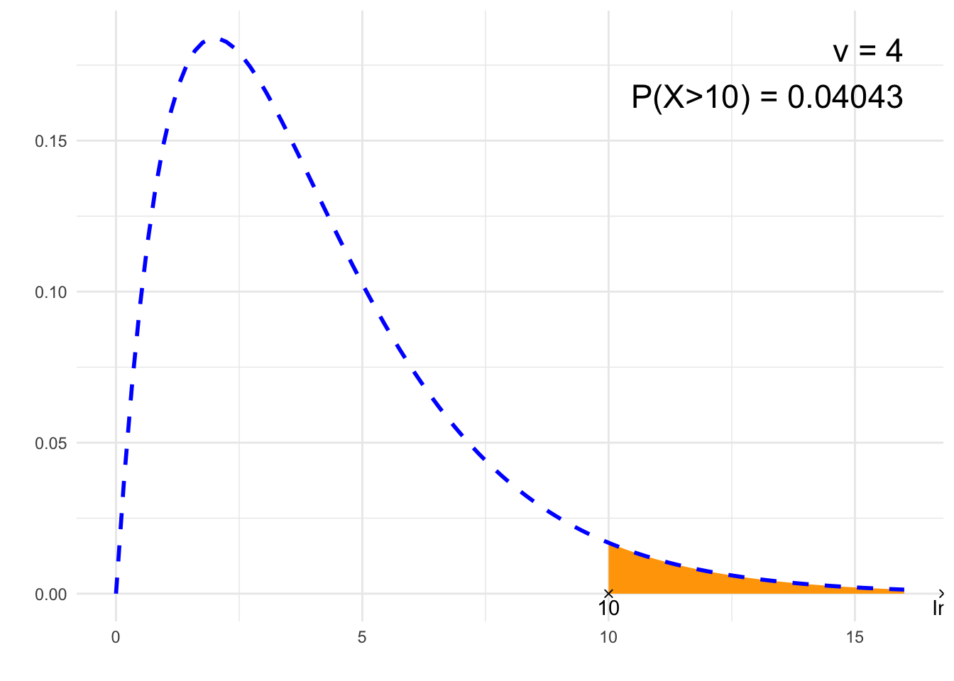
##### 2. Find x #####
# Parameter:
# Degrees of freedom:
nu <- 4

# The area under PDF:
P <- 0.05

# 'L' - left, 'R' - right, 'S' - symmetrical (middle)
typ <- 'R'

# Calculations
from <- qchisq(if(typ=='L'){0} else if(typ=='R'){1-P} else {(1-P)/2}, nu)
to <- qchisq(if(typ=='L'){P} else if(typ=='R'){1} else {1-(1-P)/2}, nu)

# P notation
if (to==Inf) {
  p=paste0("P(X>", signif(from, 6), ")")
} else if (from==-Inf) {
  p=paste0("P(X<", signif(to, 6), ")")
} else {
  p=paste0("P(", signif(from, 6), " < X < ", signif(to, 6), ")")
}
print(paste0(p, " = ", P))
## [1] "P(X>9.48773) = 0.05"# Plot
library(ggplot2)
x1=0
x2=nu*4
df<-data.frame(y=c(0, 0),
x=c(if(from==-Inf){NA}else{from}, if(to==-Inf){NA}else{to}),
label=c(if(from==-Inf){NA}else{from}, if(to==-Inf){NA}else{to}))
plt<-ggplot(NULL, aes(c(x1, x2))) +
theme_minimal() +
xlab('') +
ylab('') +
geom_area(stat = "function",
fun = function(x){dchisq(x, nu)},
fill = "orange",
xlim = c(if(from==-Inf){x1}else{from}, if(to==Inf){x2}else{to})) +
geom_line(stat = "function", fun = function(x){dchisq(x, nu)}, col = "blue", lty=2, lwd=1) +
geom_point(data = df, aes(x=x, y=y), shape=4) +
geom_text(data = df, aes(x=x, y=y, label=signif(label, 6)), vjust=1.4) +
annotate("text", label = paste0("ν = ", nu, "\n", p, " = ", P),
x = 4*nu, y = dchisq(max(nu-2,0), nu), size = 6, hjust="inward", vjust = "inward")
suppressWarnings(print(plt))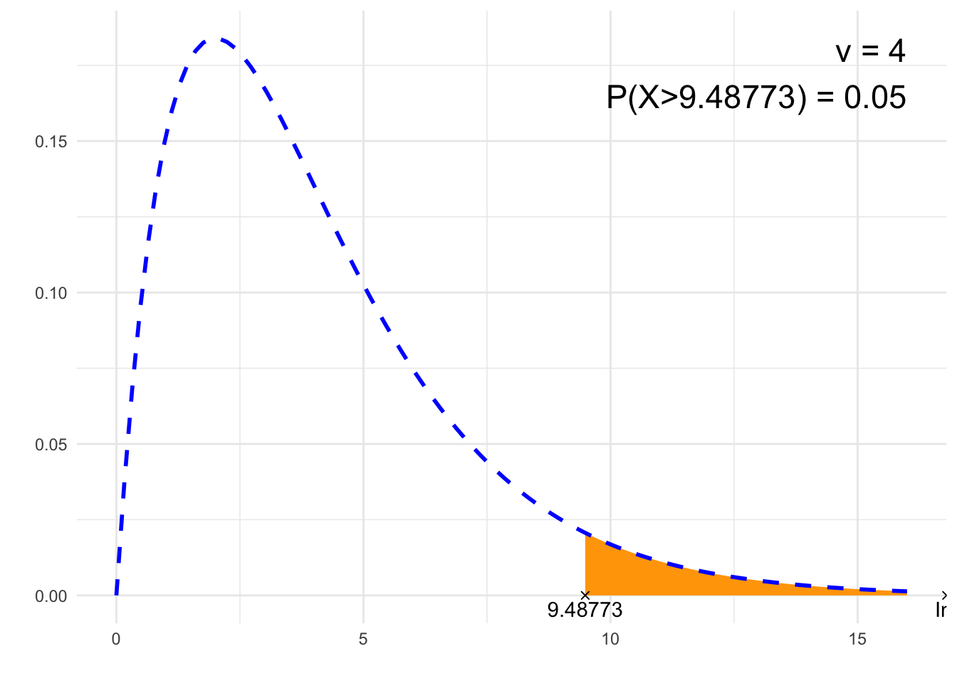
from scipy.stats import chi2
##### 1. Area under PDF #####
# Parameter:
# Degrees of freedom:
nu = 4

# Calculating the area under PDF
# from
# *for minus infinity use _from = float('-inf')
_from = 10
# to
# *for plus infinity use _to = float('inf')
_to = float('inf')

if _from > _to:
    print("!!! _From_ cannot be greater than _to_ !!!")
else:
    if _to == float('inf'):
        p = "P(X>" + str(_from) + ")"
    elif _from == float('-inf'):
        p = "P(X<" + str(_to) + ")"
    else:
        p = "P(" + str(_from) + "<X<" + str(_to) + ")"
    print(p)
    result = chi2.cdf(_to, nu) - chi2.cdf(_from, nu)
    print(result)
## P(X>10)
## 0.04042768199451274
##### 2. Find x #####

import numpy as np
from scipy.stats import chi

# Parameter:
# Degrees of freedom:
nu = 4

# The area under PDF:
P = 0.05

# 'L' - left, 'R' - right, 'S' - symmetrical (middle)
typ = 'R'

# Computation
if typ == 'L':
    _from = chi2.ppf(0, nu)
    _to = chi2.ppf(P, nu)
elif typ == 'R':
    _from = chi2.ppf(1-P, nu)
    _to = chi2.ppf(1, nu)
else:
    _from = chi2.ppf((1-P)/2, nu)
    _to = chi2.ppf(1-(1-P)/2, nu)

# P notation
if np.isinf(_to):
    p = f"P(X>{np.round(_from, 6)})"
elif np.isinf(_from):
    p = f"P(X<{np.round(_to, 6)})"
else:
    p = f"P({np.round(_from, 6)} < X < {np.round(_to, 6)})"
print(f"{p} = {P}")
## P(X>9.487729) = 0.05F distribution calculator — Google spreadsheet
##### 1. Area under PDF #####
# Parameters:
# Degrees of freedom:
nu1 <- 39
nu2 <- 34

# Calculating the area under PDF
# from
# *for minus infinity use from <- -Inf
from <- 1
# do
# *for plus infinity use to <- Inf
to <- Inf

# Data validation, calculation
if (from > to) {
  # from > to error
  print("!!! _From_ cannot be greater than _to_ !!!")
} else {

  # Probability notation

  if (to==Inf) {
    p=paste0("P(X>", from, ")")
  } else if (from==-Inf) {
    p=paste0("P(X<", to, ")")
  } else {
    p=paste0("P(", from, "<X<", to, ")")
  }
  print(p)

  # Calculating the area for the specified segment:
  result<-pf(to, nu1, nu2)-pf(from, nu1, nu2)
  print(result)
}
## [1] "P(X>1)"
## [1] 0.5030343# Plot
library(ggplot2)
x1=0
x2=qf(.999, nu1, nu2)
df<-data.frame(y=c(0, 0),
x=c(if(from==-Inf){NA}else{from}, if(to==-Inf){NA}else{to}),
label=c(if(from==-Inf){NA}else{from}, if(to==-Inf){NA}else{to}))
plt<-ggplot(NULL, aes(c(x1, x2))) +
theme_minimal() +
xlab('') +
ylab('') +
geom_line(stat = "function", fun = function(x){df(x, nu1, nu2)}, col = "blue", lty=2, lwd=1) +
geom_area(stat = "function",
fun = function(x){df(x, nu1, nu2)},
fill = "orange",
xlim = c(if(from==-Inf){x1}else{from}, if(to==Inf){x2}else{to})) +
geom_point(data = df, aes(x=x, y=y), shape=4) +
geom_text(data = df, aes(x=x, y=y, label=signif(label, 6)), vjust=1.4) +
annotate("text", label = paste0("ν1 = ", nu1, "\n", "ν2 = ", nu2, "\n", p, " = ", signif(result,4)),
x = x2, y = df(max((nu1-2)/nu1*nu2/(nu2+2),0), nu1, nu2), size = 6, hjust="inward", vjust = "inward")
suppressWarnings(print(plt))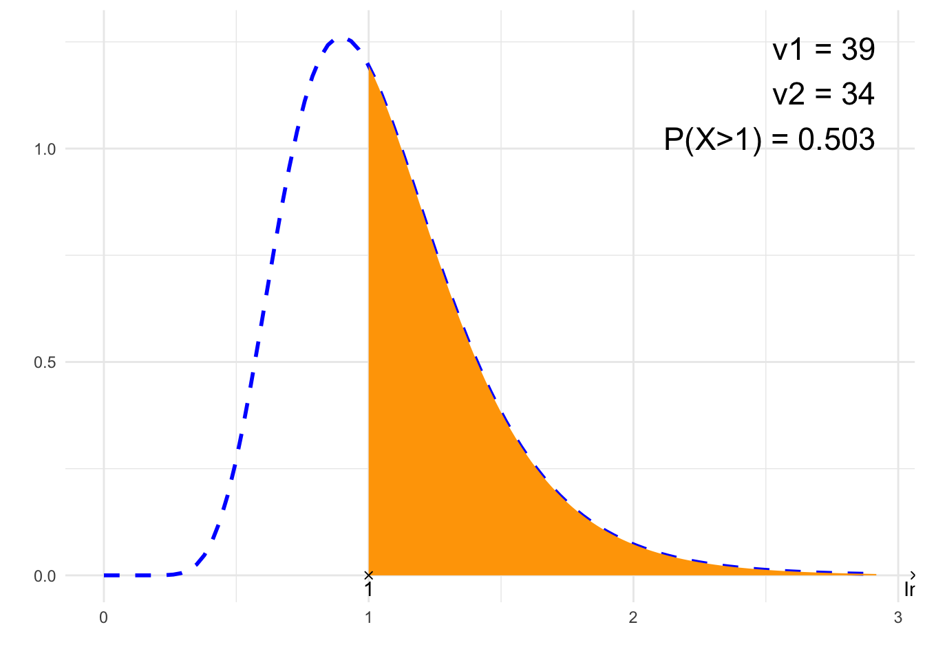
##### 2. Find x #####
# Parameters:
# Degrees of freedom:
nu1 <- 34
nu2 <- 39

# The area under PDF:
P <- 0.05

# 'L' - left, 'R' - right, 'S' - symmetrical (middle)
typ <- 'R'

# Obliczenia
from <- qf(if(typ=='L'){0} else if(typ=='R'){1-P} else {(1-P)/2}, nu1, nu2)
to <- qf(if(typ=='L'){P} else if(typ=='R'){1} else {1-(1-P)/2}, nu1, nu2)

# P notation
if (to==Inf) {
  p=paste0("P(X>", signif(from, 6), ")")
} else if (from==-Inf) {
  p=paste0("P(X<", signif(to, 6), ")")
} else {
  p=paste0("P(", signif(from, 6), " < X < ", signif(to, 6), ")")
}
print(paste0(p, " = ", P))
## [1] "P(X>1.72803) = 0.05"# Plot
library(ggplot2)
x1=0
x2=qf(.9999, nu1, nu2)
df<-data.frame(y=c(0, 0),
x=c(if(from==-Inf){NA}else{from}, if(to==-Inf){NA}else{to}),
label=c(if(from==-Inf){NA}else{from}, if(to==-Inf){NA}else{to}))
plt<-ggplot(NULL, aes(c(x1, x2))) +
theme_minimal() +
xlab('') +
ylab('') +
geom_area(stat = "function",
fun = function(x){stats::df(x, nu1, nu2)},
fill = "orange",
xlim = c(if(from==-Inf){x1}else{from}, if(to==Inf){x2}else{to})) +
geom_line(stat = "function", fun = function(x){stats::df(x, nu1, nu2)}, col = "blue", lty=2, lwd=1) +
geom_point(data = df, aes(x=x, y=y), shape=4) +
geom_text(data = df, aes(x=x, y=y, label=signif(label, 6)), vjust=1.4) +
annotate("text", label = paste0("ν1 = ", nu1, "\nν2 = ", nu2, "\n", p, " = ", P),
x = x2, y = df(max((nu1-2)/nu1*nu2/(nu2+2),0), nu1, nu2), size = 6, hjust="inward", vjust = "inward")
suppressWarnings(print(plt))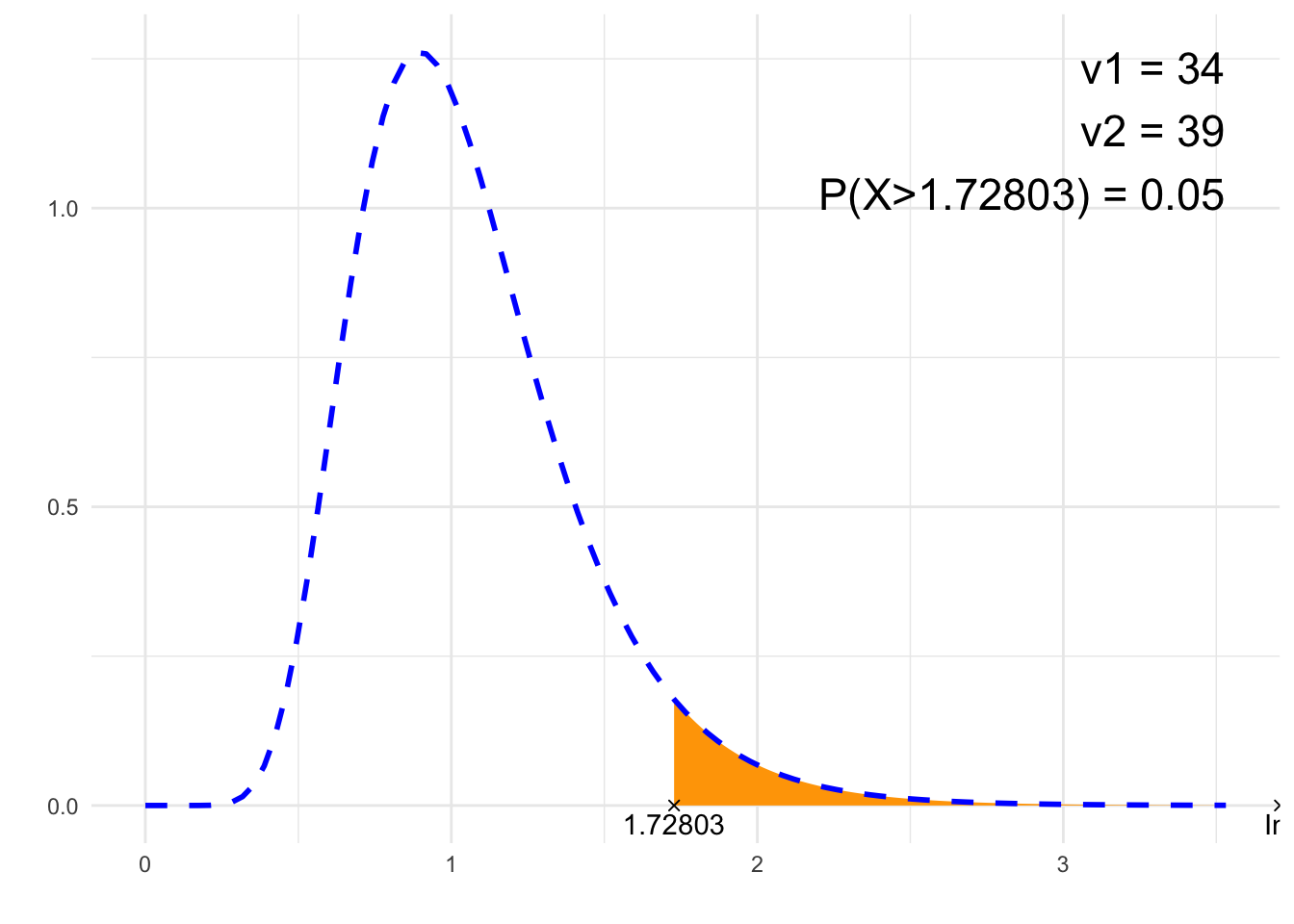
from scipy.stats import f
##### 1. Area under PDF #####
# Parameters:
# Degrees of freedom 1:
nu1 = 39
# Degrees of freedom 2:
nu2 = 34

# Calculating the area under PDF
# from
# *for minus infinity use _from = float('-inf')
_from = 1
# to
# *for plus infinity use _to = float('inf')
_to = float('inf')

if _from > _to:
    print("!!! _From_ cannot be greater than _to_ !!!")
else:
    if _to == float('inf'):
        p = "P(X>" + str(_from) + ")"
    elif _from == float('-inf'):
        p = "P(X<" + str(_to) + ")"
    else:
        p = "P(" + str(_from) + "<X<" + str(_to) + ")"
    print(p)
    result = f.cdf(_to, nu1, nu2) - f.cdf(_from, nu1, nu2)
    print(result)
## P(X>1)
## 0.503034322091588
##### 2. Find x #####

import numpy as np
from scipy.stats import chi

# Parameters:
# Degrees of freedom 1:
nu1 = 39
# Degrees of freedom 2:
nu2 = 34

# The area under PDF:
P = 0.05

# 'L' - left, 'R' - right, 'S' - symmetrical (middle)
typ = 'R'

# Obliczenia
if typ == 'L':
    _from = f.ppf(0, nu1, nu2)
    _to = f.ppf(P, nu1, nu2)
elif typ == 'R':
    _from = f.ppf(1-P, nu1, nu2)
    _to = f.ppf(1, nu1, nu2)
else:
    _from = f.ppf((1-P)/2, nu1, nu2)
    _to = f.ppf(1-(1-P)/2, nu1, nu2)

# P notation
if np.isinf(_to):
    p = f"P(X>{np.round(_from, 6)})"
elif np.isinf(_from):
    p = f"P(X<{np.round(_to, 6)})"
else:
    p = f"P({np.round(_from, 6)} < X < {np.round(_to, 6)})"
print(f"{p} = {P}")
## P(X>1.749073) = 0.05C.3 Confidence intervals
Confidence interval for a proportion — Google spreadsheet
Confidence interval for a proportion — Excel template
# Confidence interval for a proportion
# Data:
# Sample size:
n <- 160
# Number of favourable observations:
x <- 15
# Sample proportion:
phat <- x/n
# Confidence level:
conf <- 0.95

# Simple formula:
alpha <- 1 - conf
resa <- phat + c(-qnorm(1-alpha/2), qnorm(1-alpha/2)) * sqrt((1/n)*phat*(1-phat))
# Wilson score:
resw <- prop.test(x, n, conf.level = 1-alpha, correct = FALSE)$conf.int

print(paste(
  list(
    "Confidence interval - simple formula:",
    resa,
    "Confidence interval - Wilson score:",
    resw)))
## [1] "Confidence interval - simple formula:" "c(0.0485854437380776, 0.138914556261922)"
## [3] "Confidence interval - Wilson score:" "c(0.0576380069455474, 0.148912026631301)"# Using the binom package
# Sample size:
n <- 160
# Number of favourable observations:
x <- 15
# Confidence level:
conf <- 0.95
# methods="all" returns all methods, to obtain the CI with the "simple method" is method="asymptotic"
binom::binom.confint(x, n, conf.level = conf, methods = "all")## method x n mean lower upper
## 1 agresti-coull 15 160 0.09375000 0.05667743 0.1498726
## 2 asymptotic 15 160 0.09375000 0.04858544 0.1389146
## 3 bayes 15 160 0.09627329 0.05301161 0.1424125
## 4 cloglog 15 160 0.09375000 0.05494601 0.1449700
## 5 exact 15 160 0.09375000 0.05342512 0.1499102
## 6 logit 15 160 0.09375000 0.05730929 0.1496827
## 7 probit 15 160 0.09375000 0.05616008 0.1472798
## 8 profile 15 160 0.09375000 0.05506974 0.1453215
## 9 lrt 15 160 0.09375000 0.05506409 0.1453210
## 10 prop.test 15 160 0.09375000 0.05523020 0.1525939
## 11 wilson 15 160 0.09375000 0.05763801 0.1489120# Confidence interval for a proportion
# Data:
# Sample size:
n = 160
# Number of favourable observations:
x = 15
# Sample proportion:
phat = x/n
# Confidence level:
conf = 0.95
from statsmodels.stats.proportion import proportion_confint
# Simple formula:
resa = proportion_confint(x, n, alpha=1-conf, method='normal')
# Wilson score:
resw = proportion_confint(x, n, alpha=1-conf, method='wilson')
print("Confidence interval - simple formula:", resa,
"\nConfidence interval - Wilson score:", resw)## Confidence interval - simple formula: (0.048585443738077556, 0.13891455626192245)
## Confidence interval - Wilson score: (0.05763800694554742, 0.14891202663130057)Confidence interval for a mean — Google spreadsheet
Confidence interval for a mean — Excel template
# Confidence interval for the mean
# Data:
# Sample size:
n <- 24
# Sample mean:
xbar <- 183
# Population/sample standard deviation:
s <- 5.19
# Confidence level:
conf <- 0.95

alpha <- 1 - conf

# z:
ci_z <- xbar + c(-qnorm(1-alpha/2), qnorm(1-alpha/2)) * s/sqrt(n)

# t:
df<- n-1
ci_t <- xbar + c(-qt(1-alpha/2, df), qt(1-alpha/2, df)) * s/sqrt(n)

print(paste(
  list(
    "Confidence interval - z:",
    ci_z,
    "Confidence interval - t:",
    ci_t)))
## [1] "Confidence interval - z:" "c(180.923605699976, 185.076394300024)" "Confidence interval - t:"
## [4] "c(180.808455203843, 185.191544796157)"# Using raw data:
dane <- c(34.1, 35.6, 34.2, 33.9, 25.1)
test_result<-t.test(dane, conf.level = 0.99)
print(test_result$conf.int)## [1] 23.85964 41.30036
## attr(,"conf.level")
## [1] 0.99import math
import scipy.stats as stats
n = 24
xbar = 183
s = 5.19
conf = 0.95
alpha = 1 - conf
ci_z = [xbar + (-stats.norm.ppf(1-alpha/2)) * s/math.sqrt(n), xbar + (stats.norm.ppf(1-alpha/2)) * s/math.sqrt(n)]
df = n-1
ci_t = [xbar + (-stats.t.ppf(1-alpha/2, df)) * s/math.sqrt(n), xbar + (stats.t.ppf(1-alpha/2, df)) * s/math.sqrt(n)]
print("Confidence interval - z:", ci_z,
"\nConfidence interval - t:", ci_t)## Confidence interval - z: [180.92360569997632, 185.07639430002368]
## Confidence interval - t: [180.80845520384258, 185.19154479615742]# Version 2
print(stats.norm.interval(confidence=conf, loc=xbar, scale=s/math.sqrt(n)), "\n",
stats.t.interval(confidence=conf, df=df, loc=xbar, scale=s/math.sqrt(n)))## (180.92360569997632, 185.07639430002368)
## (180.80845520384258, 185.19154479615742)# Using raw data:
import numpy as np
from scipy import stats
dane = np.array([34.1, 35.6, 34.2, 33.9, 25.1])
test_result = stats.ttest_1samp(dane, popmean=np.mean(dane))
conf_int = test_result.confidence_interval(0.99)
print(conf_int)## ConfidenceInterval(low=23.85964498330358, high=41.300355016696415)C.3.1 Sample size
Sample size — Google spreadsheet
Sample size — Excel template
# Proportion estimation
# Data:
# Confidence level:
conf <- 0.99
# Margin of error (e):
e <- 0.01
# Assumed proportion (p):
p <- 0.5

# Computations
alpha <- 1 - conf
z <- -qnorm(alpha/2)

ceiling(z^2 * p * (1-p) / e^2)
## [1] 16588# Mean estimation
# Data:
# Confidence level:
conf <- 0.9
# Margin of error (e):
e <- 1
# Assumed standard deviation (sigma):
sigma <- 10
# Computation
alpha <- 1 - conf
z <- -qnorm(alpha/2)
ceiling(z^2 * sigma^2 / e^2)## [1] 271# Proportion estimation
import numpy as np
from scipy.stats import norm
# Data:
# Confidence level:
conf = 0.99
# Margin of error (e):
e = 0.01
# Assumed proportion (p):
p = 0.5
# Computations
alpha = 1 - conf
z = -norm.ppf(alpha/2)
print(np.ceil(z**2 * p * (1 - p) / e**2))## 16588.0# Mean estimation
import numpy as np
from scipy.stats import norm
# Data:
# Confidence level:
conf = 0.9
# Margin of error (e):
e = 1
# Assumed standard deviation (sigma):
sigma = 10
# Computations
alpha = 1 - conf
z = -norm.ppf(alpha / 2)
print(np.ceil(z**2 * sigma**2 / e**2))## 271.0C.4 Tests for means and proportions
C.4.1 Tests for 1 mean and 1 proportion
Tests for 1 mean and 1 proportion — Google spreadsheet
Tests for 1 mean and 1 proportion — Excel template
# Test for 1 mean
# Sample size:
n <- 38
# Sample mean:
xbar <- 184.21
# Sample/population standard deviation:
s <- 6.1034
# Significance level:
alpha <- 0.05

# Null value for the mean:
mu0 <- 179
# Alternative (sign): "<"; ">"; "<>"; "≠"
alt <- ">"

# Computations
# degrees of freedom:
df <- n-1

# critical value (t test):
crit_t <- if (alt == "<") {qt(alpha, df)} else if (alt == ">") {qt(1-alpha, df)} else {qt(1-alpha/2, df)}

# test statistic (t/z)
test_tz <- (xbar-mu0)/(s/sqrt(n))

# p-value (t test):
p.value = if(alt == ">"){1-pt(test_tz, df)} else if (alt == ">") {pt(test_tz, df)} else {2*(1-pt(abs(test_tz),df))}

# critical value (z test):
crit_z <- if (alt == "<") {qnorm(alpha)} else if (alt == ">") {qnorm(1-alpha)} else {qnorm(1-alpha/2)}

# p-value (z test):
p.value.z = if(alt == ">"){1-pnorm(test_tz)} else if (alt == ">") {pnorm(test_tz)} else {2*(1-pnorm(abs(test_tz)))}

print(c('Mean' = xbar,
        'SD' = s,
        'Sample size' = n,
        'Null hypothesis' = paste0('mu = ', mu0),
        'Alt. hypothesis' = paste0('mu ', alt, ' ', mu0),
        'Test statistic t/z' = test_tz,
        'Critical value (t test)' = crit_t,
        'P value (t test)' = p.value,
        'Critical value (z test)' = crit_z,
        'P value (z test)' = p.value.z
))
## Mean SD Sample size Null hypothesis Alt. hypothesis
## "184.21" "6.1034" "38" "mu = 179" "mu > 179"
## Test statistic t/z Critical value (t test) P value (t test) Critical value (z test) P value (z test)
## "5.26208293008297" "1.68709361959626" "3.1304551380007e-06" "1.64485362695147" "7.12162456784071e-08"# Based on raw data (test t):
# Data vector
data <- c(176.5267, 195.5237, 184.9741, 179.5349, 188.2120, 190.7425, 178.7593, 196.2744, 186.6965, 187.8559, 183.1323, 176.2569, 191.4752, 186.5975, 180.2120, 184.3434, 178.1691, 184.8852, 187.7973, 178.5013, 172.7343, 176.8545, 184.2068, 181.2395, 186.1983, 173.6317, 181.9529, 185.9135, 188.6081, 183.0285, 183.3375, 188.5512, 184.6348, 186.9657, 183.9622, 200.9014, 183.5353, 177.2538)
# Storing as an object
# Choose alternative: "two-sided" (default), "less", or "greater" and the null value (default is zero)
test_result <- t.test(data, alternative = "greater", mu = 179)
# Printing test results. Single components can be printed using for example test_result$statistic.
print(test_result)##
## One Sample t-test
##
## data: data
## t = 5.2621, df = 37, p-value = 3.13e-06
## alternative hypothesis: true mean is greater than 179
## 95 percent confidence interval:
## 182.5396 Inf
## sample estimates:
## mean of x
## 184.21# Test for 1 mean
from scipy.stats import t, norm
from math import sqrt
# Sample size:
n = 38
# Sample mean:
xbar = 184.21
# Sample/population standard deviation:
s = 6.1034
# Significance level:
alpha = 0.05
# Null value for the population mean:
mu0 = 179
# Alternative (sign): "<"; ">"; "<>"; "≠"
alt = ">"
# Calculations:
# degrees of freedom:
df = n - 1
# critical value (t test):
if alt == "<":
crit_t = t.ppf(alpha, df)
elif alt == ">":
crit_t = t.ppf(1 - alpha, df)
else:
crit_t = t.ppf(1 - alpha / 2, df)
# test statistic (t/z)
test_tz = (xbar - mu0) / (s / sqrt(n))
# p-value (t test):
if alt == ">":
p_value_t = 1 - t.cdf(test_tz, df)
elif alt == "<":
p_value_t = t.cdf(test_tz, df)
else:
p_value_t = 2 * (1 - t.cdf(abs(test_tz), df))
# critical value (z test):
if alt == "<":
crit_z = norm.ppf(alpha)
elif alt == ">":
crit_z = norm.ppf(1 - alpha)
else:
crit_z = norm.ppf(1 - alpha / 2)
# p-value (z test):
if alt == ">":
p_value_z = 1 - norm.cdf(test_tz)
elif alt == "<":
p_value_z = norm.cdf(test_tz)
else:
p_value_z = 2 * (1 - norm.cdf(abs(test_tz)))
results = {
'Mean': xbar,
'SD': s,
'Sample size': n,
'Null hypothesis': f'mu = {mu0}',
'Alt. hypothesis': f'mu {alt} {mu0}',
'Test stat. t/z': test_tz,
'Critical value t': crit_t,
'P-value (t test)': p_value_t,
'Critical value z': crit_z,
'P-value (z test)': p_value_z
}
for key, value in results.items():
print(f"{key}: {value}")## Mean: 184.21
## SD: 6.1034
## Sample size: 38
## Null hypothesis: mu = 179
## Alt. hypothesis: mu > 179
## Test stat. t/z: 5.262082930082973
## Critical value t: 1.6870936167109876
## P-value (t test): 3.1304551380006984e-06
## Critical value z: 1.6448536269514722
## P-value (z test): 7.121624567840712e-08# Raw data (t test):
import scipy.stats as stats
data = [176.5267, 195.5237, 184.9741, 179.5349, 188.2120, 190.7425, 178.7593, 196.2744, 186.6965, 187.8559, 183.1323, 176.2569, 191.4752, 186.5975, 180.2120, 184.3434, 178.1691, 184.8852, 187.7973, 178.5013, 172.7343, 176.8545, 184.2068, 181.2395, 186.1983, 173.6317, 181.9529, 185.9135, 188.6081, 183.0285, 183.3375, 188.5512, 184.6348, 186.9657, 183.9622, 200.9014, 183.5353, 177.2538]
test_result = stats.ttest_1samp(data, popmean=179, alternative='greater')
print(test_result)## TtestResult(statistic=5.262096550537936, pvalue=3.1303226590428976e-06, df=37)# Test for 1 proportion
# Sample size:
n <- 200
# Number of favourable observations:
x <- 90
# Sample proportion:
p <- x/n
# Significance level:
alpha <- 0.1
# Null proportion value:
p0 <- 0.5
# Alternative (sign): "<"; ">"; "<>"; "≠"
alt <- "≠"
alttext <- if(alt==">") {"greater"} else if(alt=="<") {"less"} else {"two.sided"}
test <- prop.test(x, n, p0, alternative=alttext, correct=FALSE)
test_z <- unname(sign(test$estimate-test$null.value)*sqrt(test$statistic))
crit_z <- if(test$alternative=="less") {qnorm(alpha)} else if(test$alternative=="greater") {qnorm(1-alpha)} else {qnorm(1-alpha/2)}
print(c('Sample proportion' = test$estimate,
'Sample size' = n,
'Null hypothesis' = paste0('p = ', test$null.value),
'Alternative hypothesis' = paste0('p ', alt, ' ', test$null.value),
'Test stat. z' = test_z,
'Test. stat. chi^2' = unname(test$statistic),
'Critical value (z)' = crit_z,
'P-value' = test$p.value
))## Sample proportion.p Sample size Null hypothesis Alternative hypothesis Test stat. z
## "0.45" "200" "p = 0.5" "p ≠ 0.5" "-1.4142135623731"
## Test. stat. chi^2 Critical value (z) P-value
## "2" "1.64485362695147" "0.157299207050284"# Test for 1 proportion
from statsmodels.stats.proportion import proportions_ztest
# Sample size:
n = 200
# Number of favourable observations:
x = 90
# Sample proportion:
p = x/n
# Significance level:
alpha = 0.1
# Null proportion value:
p0 = 0.5
# Alternative hypothesis (sign): "<"; ">"; "<>"; "≠"
alt = "≠"
if alt == ">":
alttext = "larger"
elif alt == "<":
alttext = "smaller"
else:
alttext = "two-sided"
test_result = proportions_ztest(count = x, nobs = n, value = p0, alternative = alttext, prop_var=p0)
print("Test statistic (z):", test_result[0], "\np-value:", test_result[1])## Test statistic (z): -1.4142135623730947
## p-value: 0.15729920705028533C.4.2 Tests and confidence intervals for 2 means
Test and confidence intervals for 2 means — Google spreadsheet
Test and confidence intervals for 2 means — Excel template
# Test z for 2 means
# Sample 1 size:
n1 <- 100
# Sample 1 mean:
xbar1 <- 76.5
# Sample 1 standard deviation:
s1 <- 38.0

# Sample 2 size:
n2 <- 100
# Sample 2 mean:
xbar2 <- 88.1
# Sample 2 standard deviation:
s2 <- 40.0

# Significance level:
alpha <- 0.05

# Null value (usually 0):
mu0 <- 0

# Alternative (sign): "<"; ">"; "<>"; "≠"
alt <- "<"

# Calculations:
# Z test statistic:
test_z <- (xbar1-xbar2-mu0)/sqrt(s1^2/n1+s2^2/n2)

# Z test critical value:
crit_z <- if (alt == "<") {qnorm(alpha)} else if (alt == ">") {qnorm(1-alpha)} else {qnorm(1-alpha/2)}

# Z test p-value:
p.value.z = if(alt == ">"){1-pnorm(test_z)} else if (alt == "<") {pnorm(test_z)} else {2*(1-pnorm(abs(test_z)))}

print(c('Mean 1' = xbar1,
        'SD 1' = s1,
        'Sample 1 size' = n1,
        'Mean 2' = xbar2,
        'SD 2' = s2,
        'Sample 2 size' = n2,
        'Null hypothesis' = paste0('mu1-mu2 = ', mu0),
        'Alternative hypothesis' = paste0('mu1-mu2 ', alt, ' ', mu0),
        'Z test statistic' = test_z,
        'Z test critical value' = crit_z,
        'Z test p-value' = p.value.z
))
## Mean 1 SD 1 Sample 1 size Mean 2 SD 2
## "76.5" "38" "100" "88.1" "40"
## Sample 2 size Null hypothesis Alternative hypothesis Z test statistic Z test critical value
## "100" "mu1-mu2 = 0" "mu1-mu2 < 0" "-2.1024983574238" "-1.64485362695147"
## Z test p-value
## "0.0177548216928505"# Test z for 2 means
# Sample 1 size:
n1 <- 14
# Sample 1 mean:
xbar1 <- 185.2142
# Sample 1 standard deviation:
s1 <- 7.5261
# Sample 2 size:
n2 <- 19
# Sample 2 mean:
xbar2 <- 184.8421
# Sample 2 standard deviation:
s2 <- 5.0471
# Significance level:
alpha <- 0.05
# Null value (usually 0):
mu0 <- 0
# Alternative (sign): "<"; ">"; "<>"; "≠"
alt <- "≠"
# Assume equal variances? (TRUE/FALSE):
eqvar <- FALSE
# Calculations
# Pooled standard deviation:
sp <- sqrt(((n1-1)*s1^2+(n2-1)*s2^2)/(n1+n2-2))
# T test statistic:
test_t <- if(eqvar) {(xbar1-xbar2-mu0)/sqrt(sp^2*(1/n1+1/n2))} else {(xbar1-xbar2-mu0)/sqrt(s1^2/n1+s2^2/n2)}
# Degrees of freedom:
df<-if(eqvar) {n1+n2-2} else {(s1^2/n1+s2^2/n2)^2/((s1^2/n1)^2/(n1-1)+(s2^2/n2)^2/(n2-1))}
# T critical value:
crit_t <- if (alt == "<") {qt(alpha, df)} else if (alt == ">") {qt(1-alpha, df)} else {qt(1-alpha/2, df)}
# T test p-value:
p.value.t = if(alt == ">"){1-pt(test_t, df)} else if (alt == ">") {pt(test_t, df)} else {2*(1-pt(abs(test_t),df))}
print(c('Mean 1' = xbar1,
'SD 1' = s1,
'Sample 1 size' = n1,
'Mean 2' = xbar2,
'SD 2' = s2,
'Sample size 2' = n2,
'Null hypothesis' = paste0('mu1-mu2 = ', mu0),
'Alt. hypothesis' = paste0('mu1-mu2 ', alt, ' ', mu0),
'T test statistic' = test_t,
'T test critival value' = crit_t,
'T test p-value' = p.value.t
))## Mean 1 SD 1 Sample 1 size Mean 2 SD 2
## "185.2142" "7.5261" "14" "184.8421" "5.0471"
## Sample size 2 Null hypothesis Alt. hypothesis T test statistic T test critival value
## "19" "mu1-mu2 = 0" "mu1-mu2 ≠ 0" "0.160325899672522" "2.07753969816904"
## T test p-value
## "0.874131604618"# Using raw data (t test)
# Two data vectors:
data1 <- c(1.2, 3.1, 1.7, 2.8, 3.0)
data2 <- c(4.2, 2.7, 3.6, 3.9)
# Storing test results as an object.
# Choose alternative: "two-sided" (default), "less", or "greater" and the the equality of variances assumption TRUE/FALSE (default is FALSE)
test_result <- t.test(data1, data2, alternative="two.sided", var.equal = TRUE)
# Printing test results. Single components can be printed using for example test_result$statistic.
print(test_result)##
## Two Sample t-test
##
## data: data1 and data2
## t = -2.3887, df = 7, p-value = 0.04826
## alternative hypothesis: true difference in means is not equal to 0
## 95 percent confidence interval:
## -2.46752406 -0.01247594
## sample estimates:
## mean of x mean of y
## 2.36 3.60import math
from scipy.stats import norm
# Test z for 2 means
# Sample 1 size:
n1 = 100
# Sample 1 mean:
xbar1 = 76.5
# Sample 1 standard deviation:
s1 = 38.0
# Sample 2 size:
n2 = 100
# Sample 2 mean:
xbar2 = 88.1
# Sample 2 standard deviation:
s2 = 40.0
# Significance level:
alpha = 0.05
# Null value (usually 0):
mu0 = 0
# Alternative (sign): "<"; ">"; "<>"/"≠"
alt = "<"
# Calculations:
# Z test statistic:
test_z = (xbar1 - xbar2 - mu0) / math.sqrt(s1**2 / n1 + s2**2 / n2)
# Z test critical value:
if alt == "<":
crit_z = norm.ppf(alpha)
elif alt == ">":
crit_z = norm.ppf(1 - alpha)
else:
crit_z = norm.ppf(1 - alpha / 2)
# Z test p-value:
if alt == ">":
p_value_z = 1 - norm.cdf(test_z)
elif alt == "<":
p_value_z = norm.cdf(test_z)
else:
p_value_z = 2 * (1 - norm.cdf(abs(test_z)))
results = {
'Mean 1': xbar1,
'SD 1': s1,
'Sample 1 size': n1,
'Mean 2': xbar2,
'SD 2': s2,
'Sample 2 size': n2,
'Null hypothesis': f'mu1-mu2 = {mu0}',
'Alt. hypothesis': f'mu1-mu2 {alt} {mu0}',
'Z test statistic': test_z,
'Z test critical value': crit_z,
'Z test p-value': p_value_z
}
for key, value in results.items():
print(f"{key}: {value}")## Mean 1: 76.5
## SD 1: 38.0
## Sample 1 size: 100
## Mean 2: 88.1
## SD 2: 40.0
## Sample 2 size: 100
## Null hypothesis: mu1-mu2 = 0
## Alt. hypothesis: mu1-mu2 < 0
## Z test statistic: -2.102498357423799
## Z test critical value: -1.6448536269514729
## Z test p-value: 0.017754821692850486# T test for 2 means
from scipy.stats import t
# Sample 1 size:
n1 = 14
# Sample 1 mean:
xbar1 = 185.2142
# Sample 1 standard deviation:
s1 = 7.5261
# Sample 2 size:
n2 = 19
# Sample 2 mean:
xbar2 = 184.8421
# Sample 2 standard deviation:
s2 = 5.0471
# Poziom istotności:
alpha = 0.05
# Null value (usually 0):
mu0 = 0
# Alternative (sign): "<"; ">"; "<>"/"≠"
alt = "≠"
# Assume equal variances? (True/False):
eqvar = False
# Calculations
# Pooled standard deviation:
sp = math.sqrt(((n1 - 1) * s1**2 + (n2 - 1) * s2**2) / (n1 + n2 - 2))
# T test statistic and degrees of freedom:
if eqvar:
test_t = (xbar1 - xbar2 - mu0) / math.sqrt(sp**2 * (1/n1 + 1/n2))
df = n1 + n2 - 2
else:
test_t = (xbar1 - xbar2 - mu0) / math.sqrt(s1**2 / n1 + s2**2 / n2)
df = (s1**2 / n1 + s2**2 / n2)**2 / ((s1**2 / n1)**2 / (n1 - 1) + (s2**2 / n2)**2 / (n2 - 1))
# T test critival value:
if alt == "<":
crit_t = t.ppf(alpha, df)
elif alt == ">":
crit_t = t.ppf(1 - alpha, df)
else:
crit_t = t.ppf(1 - alpha / 2, df)
# T test p-value:
if alt == ">":
p_value_t = 1 - t.cdf(test_t, df)
elif alt == "<":
p_value_t = t.cdf(test_t, df)
else:
p_value_t = 2 * (1 - t.cdf(abs(test_t), df))
results = {
'Mean 1': xbar1,
'SD 1': s1,
'Sample 1 size': n1,
'Mean 2': xbar2,
'SD 2': s2,
'Sample 2 size': n2,
'Null hypothesis': f'mu1-mu2 = {mu0}',
'Alt. hypothesis': f'mu1-mu2 {alt} {mu0}',
'Z test statistic': test_t,
'Z test critical value': crit_t,
'Z test p-value': p_value_t
}
for key, value in results.items():
print(f"{key}: {value}")## Mean 1: 185.2142
## SD 1: 7.5261
## Sample 1 size: 14
## Mean 2: 184.8421
## SD 2: 5.0471
## Sample 2 size: 19
## Null hypothesis: mu1-mu2 = 0
## Alt. hypothesis: mu1-mu2 ≠ 0
## Z test statistic: 0.16032589967252212
## Z test critical value: 2.0775396981690264
## Z test p-value: 0.8741316046180003
# Using raw data (t test)
from scipy.stats import ttest_ind, t

# Two data vectors
data1 = [1.2, 3.1, 1.7, 2.8, 3.0]
data2 = [4.2, 2.7, 3.6, 3.9]

# Storing test results as an object.
# Choose alternative: "two-sided" (default), "less", or "greater" and the the equality of variances assumption True/False (default is False)
test_result = ttest_ind(data1, data2, alternative='two-sided', equal_var=True)

print(test_result)
## TtestResult(statistic=-2.3886571085065054, pvalue=0.04826397365151946, df=7.0)C.4.3 Tests and confidence intervals for 2 proportions
Tests and confidence intervals for 2 proportions — Google spreadsheet
Tests and confidence intervals for 2 proportions — Excel template
# Test for 2 proportions
# Sample 1 size:
n1 <- 24
# Number of favourable observations in sample 1:
x1 <- 21
# Sample 1 proportion:
phat1 <- x1/n1
# Sample 2 size:
n2 <- 24
# Number of favourable observations in sample 2:
x2 <- 14
# Sample 2 proportion:
phat2 <- x2/n2


# Significance level:
alpha <- 0.05
# Alternative (sign): "<"; ">"; "<>"/"≠"
alt <- ">"

alttext <- if(alt==">") {"greater"} else if(alt=="<") {"less"} else {"two.sided"}

test <- prop.test(c(x1, x2), c(n1, n2), alternative=alttext, correct=FALSE)
test_z <- unname(-sign(diff(test$estimate))*sqrt(test$statistic))
crit_z <- if(test$alternative=="less") {qnorm(alpha)} else if(test$alternative=="greater") {qnorm(1-alpha)} else {qnorm(1-alpha/2)}

print(c('Sample proportions ' = test$estimate,
        'Sample sizes ' = c(n1, n2),
        'Null hypothesis' = paste0('p1-p2 = ', 0),
        'Alt. hypothesis' = paste0('p1-p2 ', alt, ' ', 0),
        'Z test statistic' = test_z,
        'Chi^2 test statistic' = unname(test$statistic),
        'Z test critival value' = crit_z,
        'Chi^2 test critival value' = crit_z^2,
        'P-value' = test$p.value
))
## Sample proportions .prop 1 Sample proportions .prop 2 Sample sizes 1 Sample sizes 2
## "0.875" "0.583333333333333" "24" "24"
## Null hypothesis Alt. hypothesis Z test statistic Chi^2 test statistic
## "p1-p2 = 0" "p1-p2 > 0" "2.27359424023522" "5.16923076923077"
## Z test critival value Chi^2 test critival value P-value
## "1.64485362695147" "2.70554345409541" "0.0114951970462325"from statsmodels.stats.proportion import proportions_ztest
from scipy.stats import norm, chi2_contingency
import numpy as np
n1 = 24
x1 = 21
phat1 = x1 / n1
n2 = 24
x2 = 14
phat2 = x2 / n2
alpha = 0.05
alt = ">"
if alt == ">":
alttext = "larger"
elif alt == "<":
alttext = "smaller"
else:
alttext = "two-sided"
test_result = proportions_ztest(count = np.array([x1, x2]), nobs = np.array([n1, n2]), alternative = alttext)
print("Z test statistic:", test_result[0],
"\np-value:", test_result[1])## Z test statistic: 2.2735942402352203
## p-value: 0.011495197046232447C.5 Chi-square test
Chi-square test — Google spreadsheet
Chi-square test — Excel template
# Indepenence/homogeneity test

# Data matrix

# Input vector
m <- c(
  21, 14,
  3, 10
)

# Number of rows in the data matrix
nrow <- 2

# Significance level
alpha <- 0.05

# Transformation of the vector to a matrix
m <- matrix(data=m, nrow=nrow, byrow=TRUE)

# Chi-square test without Yates' correction
test_chi <- chisq.test(m, correct=FALSE)

# Chi-square test with Yates' correction for 2x2 tables
test_chi_corrected <- chisq.test(m)

# G test
test_g <- AMR::g.test(m)

# Exact Fisher test
exact_fisher<-fisher.test(m)

print(c('Degrees of freedom' = test_chi$parameter,
        'Critical value' = qchisq(1-alpha, test_chi$parameter),
        'Chi^2 statistic' = unname(test_chi$statistic),
        'Chi^2 test p-value' = test_chi$p.value,
        "Cramér's V" = unname(sqrt(test_chi$statistic/sum(m)/min(dim(m)-1))),
        'Phi coefficient (2x2 tables)' = if(all(dim(m)==2)) {psych::phi(m, digits=10)},
        "Chi^2 with Yates' correction test statistic" = unname(test_chi_corrected$statistic),
        "Chi^2 with Yates' correction p-value" = test_chi_corrected$p.value,
        'G statistic' = unname(test_g$statistic),
        'G test p-value' = test_g$p.value,
        'Exact Fisher test p-value' = exact_fisher$p.value
))
## Degrees of freedom.df Critical value
## 1.00000000 3.84145882
## Chi^2 statistic Chi^2 test p-value
## 5.16923077 0.02299039
## Cramér's V Phi coefficient (2x2 tables)
## 0.32816506 0.32816506
## Chi^2 with Yates' correction test statistic Chi^2 with Yates' correction p-value
## 3.79780220 0.05131990
## G statistic G test p-value
## 5.38600494 0.02029889
## Exact Fisher test p-value
## 0.04899141# Goodness-of-fit chi-square test
# Observed frequencies:
observed <- c(70, 10, 20)
# Expected frequencies:
expected <- c(80, 10, 10)
# Just in case: Adjustment of the expected frequencies so that their sum is equal to the sum of the observed frequencies:
expected <- expected / sum(expected) * sum(observed)
# Significance level
alpha <- 0.05
test_chi <- chisq.test(x = observed, p = expected, rescale.p = TRUE)
test_g <- AMR::g.test(x = observed, p = expected, rescale.p = TRUE)
print(c('Degrees of freedom' = test_chi$parameter,
'Critical value' = qchisq(1-alpha, test_chi$parameter),
'Chi^2 statistic' = unname(test_chi$statistic),
'p-value (chi-square test)' = test_chi$p.value,
'G statistic' = unname(test_g$statistic),
'p-value (G test)' = test_g$p.value
))## Degrees of freedom.df Critical value Chi^2 statistic p-value (chi-square test)
## 2.000000000 5.991464547 11.250000000 0.003606563
## G statistic p-value (G test)
## 9.031492255 0.010935443# Indepenence/homogeneity test
import numpy as np
import scipy.stats as stats
from scipy.stats import chi2
from statsmodels.stats.contingency_tables import Table2x2
# Data matrix
m = np.array([
[21, 14],
[3, 10]
])
alpha = 0.05
# Chi-square test without Yates' correction
test_chi = stats.chi2_contingency(m, correction=False)
# Chi-square test with Yates' correction for 2x2 tables
test_chi_corrected = stats.chi2_contingency(m)
# G test
g, p, dof, expected = stats.chi2_contingency(m, lambda_="log-likelihood")
# Exact Fisher test
exact_fisher = stats.fisher_exact(m)
# Cramér's V
cramers_v = np.sqrt(test_chi[0] / m.sum() / min(m.shape[0]-1, m.shape[1]-1))
# Phi coefficient (2x2 tables)
phi_coefficient = None
if m.shape == (2, 2):
phi_coefficient = cramers_v*np.sign(np.diagonal(m).prod()-np.diagonal(np.fliplr(m)).prod())
# Results
results = {
'Number of degrees of freedom': test_chi[2],
'Critical value': chi2.ppf(1-alpha, test_chi[2]),
'Chi-square statistic': test_chi[0],
'p-value (chi-square test)': test_chi[1],
"Cramer\'s V": cramers_v,
'Phi coefficient (for 2x2 table)': phi_coefficient,
"Chi-square statistic with Yates' correction": test_chi_corrected[0],
"p-value (chi-square test with Yates' correction)": test_chi_corrected[1],
'G statistic': g,
'p-value (G test)': p,
'p-value (Fisher’s exact test)': exact_fisher[1]
}
for key, value in results.items():
print(f"{key}: {value}")## Number of degrees of freedom: 1
## Critical value: 3.841458820694124
## Chi-square statistic: 5.169230769230769
## p-value (chi-square test): 0.022990394092464842
## Cramer's V: 0.3281650616569468
## Phi coefficient (for 2x2 table): 0.3281650616569468
## Chi-square statistic with Yates' correction: 3.7978021978021976
## p-value (chi-square test with Yates' correction): 0.05131990358807137
## G statistic: 3.9106978537750194
## p-value (G test): 0.04797967015430134
## p-value (Fisher’s exact test): 0.048991413058947844# Goodness-of-fit chi-square test
from scipy.stats import chisquare, chi2
import numpy as np
# Liczebności rzeczywiste:
observed = np.array([70, 10, 20])
# Liczebności oczekiwane:
expected = np.array([80, 10, 10])
# Ewentualna korekta liczebności oczekiwanych, żeby ich suma była na pewno równa sumie rzeczywistych:
expected = expected / expected.sum() * observed.sum()
# Test chi-kwadrat:
chi_stat, chi_p = chisquare(f_obs=observed, f_exp=expected)
# Liczba stopni swobody:
df = len(observed) - 1
# Poziom istotności:
alpha = 0.05
# Wartość krytyczna:
critical_value = chi2.ppf(1 - alpha, df)
# Test G:
from scipy.stats import power_divergence
g_stat, g_p = power_divergence(f_obs=observed, f_exp=expected, lambda_="log-likelihood")
# Wyniki
results = {
'Liczba stopni swobody': df,
'Wartość krytyczna': critical_value,
'Statystyka chi^2': chi_stat,
'Wartość p (test chi-kwadrat)': chi_p,
'Statystyka G': g_stat,
'Wartość p (test G)': g_p
}
for key, value in results.items():
print(f"{key}: {value}")## Liczba stopni swobody: 2
## Wartość krytyczna: 5.991464547107979
## Statystyka chi^2: 11.25
## Wartość p (test chi-kwadrat): 0.0036065631360157305
## Statystyka G: 9.031492254964643
## Wartość p (test G): 0.010935442847719828C.6 ANOVA i test Levene'a
ANOVA — Google spreadsheet
ANOVA — Excel template
# Example data
group <- as.factor(c(rep("A",7), rep("B",7), rep("C",7), rep("D",7)))
result <- c(51, 87, 50, 48, 79, 61, 53, 82, 91, 92, 80, 52, 79, 73,
            79, 84, 74, 98, 63, 83, 85, 85, 80, 65, 71, 67, 51, 80)
data<-data.frame(group, result)

#To view the data, you can run: View(data)
#To write the data to a text file, you can run: write.csv2(data, "data.csv")
#To load data from a text file, you can run: read.csv2("data.csv")

# Summary table
library(dplyr)
data %>%
  group_by(group) %>%
  summarize(n=n(), suma = sum(result), srednia = mean(result), odch_st=sd(result), mediana = median(result)) %>%
  data.frame() -> summary_table

# ANOVA table
model<-aov(result~group, data=data)
anova_summary<-summary(model)

# Levene's test (Brown-Forsythe test)
levene_result<-car::leveneTest(result~group, data=data)

# Tukey's procedure
tukey_result<-TukeyHSD(x=model, conf.level=0.95)

print(list(`Summary` = summary_table, `ANOVA table` = anova_summary, `Levene test` = levene_result,
           `Tukey HSD` = tukey_result))
## $Summary
## group n suma srednia odch_st mediana
## 1 A 7 429 61.28571 15.56400 53
## 2 B 7 549 78.42857 13.45185 80
## 3 C 7 566 80.85714 10.76148 83
## 4 D 7 499 71.28571 11.61485 71
##
## $`ANOVA table`
## Df Sum Sq Mean Sq F value Pr(>F)
## group 3 1620 539.8 3.204 0.0412 *
## Residuals 24 4043 168.5
## ---
## Signif. codes: 0 '***' 0.001 '**' 0.01 '*' 0.05 '.' 0.1 ' ' 1
##
## $`Levene test`
## Levene's Test for Homogeneity of Variance (center = median)
## Df F value Pr(>F)
## group 3 0.1898 0.9023
## 24
##
## $`Tukey HSD`
## Tukey multiple comparisons of means
## 95% family-wise confidence level
##
## Fit: aov(formula = result ~ group, data = data)
##
## $group
## diff lwr upr p adj
## B-A 17.142857 -1.996412 36.282127 0.0905494
## C-A 19.571429 0.432159 38.710698 0.0437429
## D-A 10.000000 -9.139270 29.139270 0.4870470
## C-B 2.428571 -16.710698 21.567841 0.9849136
## D-B -7.142857 -26.282127 11.996412 0.7340659
## D-C -9.571429 -28.710698 9.567841 0.5237024import pandas as pd
import numpy as np
from scipy import stats
import statsmodels.api as sm
from statsmodels.formula.api import ols
from statsmodels.stats.multicomp import pairwise_tukeyhsd
from statsmodels.stats.anova import anova_lm
# Data frame
group = ['A']*7 + ['B']*7 + ['C']*7 + ['D']*7
result = [51, 87, 50, 48, 79, 61, 53,
82, 91, 92, 80, 52, 79, 73,
79, 84, 74, 98, 63, 83, 85,
85, 80, 65, 71, 67, 51, 80]
data = pd.DataFrame({'group': group, 'result': result})
# Summary table
summary_table = data.groupby('group')['result'].agg(['count', 'sum', 'mean', 'std', 'median']).reset_index()
summary_table.columns = ['group', 'n', 'sum', 'mean', 'sd', 'median']
# ANOVA
model = ols('result ~ group', data=data).fit()
anova_summary = anova_lm(model, typ=2)
# Levene's test (Brown-Forsythe test)
levene_result = stats.levene(data['result'][data['group'] == 'A'],
data['result'][data['group'] == 'B'],
data['result'][data['group'] == 'C'],
data['result'][data['group'] == 'D'])
# Tukey's HSD
tukey_result = pairwise_tukeyhsd(endog=data['result'], groups=data['group'], alpha=0.05)
print('Summary:\n\n', summary_table, '\n\nANOVA:\n\n', anova_summary, '\n\nLevene\'s test:\n\n', levene_result,
'\n\nTukey HSD:\n\n', tukey_result)## Summary:
##
## group n sum mean sd median
## 0 A 7 429 61.285714 15.564000 53.0
## 1 B 7 549 78.428571 13.451854 80.0
## 2 C 7 566 80.857143 10.761483 83.0
## 3 D 7 499 71.285714 11.614851 71.0
##
## ANOVA:
##
## sum_sq df F PR(>F)
## group 1619.535714 3.0 3.204282 0.041204
## Residual 4043.428571 24.0 NaN NaN
##
## Levene's test:
##
## LeveneResult(statistic=0.18975139523084725, pvalue=0.9023335775328473)
##
## Tukey HSD:
##
## Multiple Comparison of Means - Tukey HSD, FWER=0.05
## =====================================================
## group1 group2 meandiff p-adj lower upper reject
## -----------------------------------------------------
## A B 17.1429 0.0905 -1.9964 36.2821 False
## A C 19.5714 0.0437 0.4322 38.7107 True
## A D 10.0 0.487 -9.1393 29.1393 False
## B C 2.4286 0.9849 -16.7107 21.5678 False
## B D -7.1429 0.7341 -26.2821 11.9964 False
## C D -9.5714 0.5237 -28.7107 9.5678 False
## -----------------------------------------------------C.7 Nonparametric tests
Nonparametric tests — Google spreadsheet
Nonparametric tests — Excel template
# Runs test
# Example data
vHT <- "HHTHTTTHHTHTTHHTHTHHTHTHHHTTHTHTHTTHHTTTTHHTHHTTHTHTTHTHHHT"

# Transforming into a vector of 0s and 1s
v01 <- 1*(unlist(strsplit(vHT, ""))=="H")

# Test
DescTools::RunsTest(v01)
##
## Runs Test for Randomness
##
## data: v01
## z = 1.8413, runs = 38, m = 29, n = 30, p-value = 0.06557
## alternative hypothesis: true number of runs is not equal the expected number# Mann-Whitney test
# Data (example):
p1<-c(24, 25, 21, 22, 23, 18, 17, 28, 24, 27, 21, 23)
p2<-c(20, 23, 21, 25, 18, 17, 18, 24, 20, 24, 23, 19)
# Test
# with parameters: wilcox.test(p1, p2, correct=TRUE, exact=FALSE)
wilcox.test(p1, p2)##
## Wilcoxon rank sum test with continuity correction
##
## data: p1 and p2
## W = 94, p-value = 0.2114
## alternative hypothesis: true location shift is not equal to 0# Wilcoxon paired test
# Data (example):
p1<-c(24, 25, 21, 22, 23, 18, 17, 28, 24, 27, 21, 23)
p2<-c(20, 23, 21, 25, 18, 17, 18, 24, 20, 24, 23, 19)
# Test:
# parameters: wilcox.test(p2, p1, paired=TRUE, correct=FALSE, exact=FALSE, alternative="two.sided")
wilcox.test(p1, p2, paired=TRUE)##
## Wilcoxon signed rank test with continuity correction
##
## data: p1 and p2
## V = 55.5, p-value = 0.04898
## alternative hypothesis: true location shift is not equal to 0# Kruskal-Wallis test
# Data (example):
df<-data.frame(A = c(7,8,9,9,10,11), B = c(12,13,14,14,15,16))
df2 <- tidyr::gather(df)
# Test:
kruskal.test(value ~ key, data = df2)##
## Kruskal-Wallis rank sum test
##
## data: value by key
## Kruskal-Wallis chi-squared = 8.3662, df = 1, p-value = 0.003823import numpy as np
import pandas as pd
from scipy.stats import wilcoxon, kruskal, mannwhitneyu
from statsmodels.stats.proportion import proportions_ztest
# Runs test
# Example data
vHT = "HHTHTTTHHTHTTHHTHTHHTHTHHHTTHTHTHTTHHTTTTHHTHHTTHTHTTHTHHHT"
# Transforming into a vector of 0s and 1s
v01 = np.array([1 if char == 'H' else 0 for char in vHT])
# Calculations
def getRuns(l):
import itertools
# return len([sum(1 for _ in r) for _, r in itertools.groupby(l)])
return sum(1 for _ in itertools.groupby(l))
r = getRuns(v01)
n = len(v01)
n1 = sum(v01)
n0 = n - n1
mu_r = (2 * n0 * n1 / n) + 1
sigma_r = np.sqrt((2 * n0 * n1 * (2 * n0 * n1 - n)) / (n ** 2 * (n - 1)))
z = (r-mu_r-np.sign(r-mu_r)/2)/sigma_r
p_value = 2 * (1 - norm.cdf(abs(z)))
print("z =", z, "p-value =", p_value)## z = 1.8413274595803757 p-value = 0.0655735860394191# Mann-Whitney test
# Data (example):
p1 = np.array([24, 25, 21, 22, 23, 18, 17, 28, 24, 27, 21, 23])
p2 = np.array([20, 23, 21, 25, 18, 17, 18, 24, 20, 24, 23, 19])
# Test
mannwhitneyu(p1, p2)## MannwhitneyuResult(statistic=94.0, pvalue=0.21138945901258455)# Wilcoxon paired test
# Data (example):
p1 = np.array([24, 25, 21, 22, 23, 18, 17, 28, 24, 27, 21, 23])
p2 = np.array([20, 23, 21, 25, 18, 17, 18, 24, 20, 24, 23, 19])
# Test
wilcoxon(p1, p2)## WilcoxonResult(statistic=10.5, pvalue=0.044065400736826854)# Kruskal-Wallis test
# Data (example):
df = pd.DataFrame({'A': [7, 8, 9, 9, 10, 11], 'B': [12, 13, 14, 14, 15, 16]})
df2 = df.melt()
# Test
kruskal(*[group["value"].values for name, group in df2.groupby("variable")])## KruskalResult(statistic=8.366197183098597, pvalue=0.0038226470545864484)C.8 Other tests
C.8.1 Regression
Simple regression — Google spreadsheet
Simple regression — Excel template
Multiple regression — Google spreadsheet
Multiple regression — Excel template
C.8.2 Normality check
Normality check — Google spreadsheet
Normality check — Excel template
# Normality check
# Data
data<-c(76, 62, 55, 62, 56, 64, 44, 56, 94, 37, 72, 85, 72, 71, 60, 61, 64, 71, 69, 70, 64, 59, 71, 65, 84)
# Sample mean
m<-mean(data)
# Sample standard deviation
s<-sd(data)
# Skewness
skew<-e1071::skewness(data, type=2)
# Kurtosis
kurt<-e1071::kurtosis(data, type=2)
# IQR/s ratio
IQR_to_s<-IQR(data)/s
# proportion of observations within 1 sd from the mean
within1s<-mean(abs(data-m)<s)
# proportion of observations within 2 sds from the mean
within2s<-mean(abs(data-m)<2*s)
# proportion of observations within 3 sd from the mean
within3s<-mean(abs(data-m)<3*s)
# Shapiro-Wilk test
SW_res<-shapiro.test(data)
# Jarque-Bera test
JB_res<-tseries::jarque.bera.test(data)
# Anderson-Darling test
AD_res<-nortest::ad.test(data)
# Kolmogorov-Smirnov test
KS_res <- ks.test(data, function(x){pnorm(x, mean(data), sd(data))})

# Results
print(c('Mean' = m,
        'St. deviation' = s,
        'Sample size' = length(data),
        'Skewnes (~=0?)' = skew,
        'Kurtosis (~=0?)' = kurt,
        'IQR/s (~=1,3?)' = IQR_to_s,
        '68% rule' = within1s*100,
        '95% rule' = within2s*100,
        '100% rule' = within3s*100,
        'Test stat. - SW test' = SW_res$statistic,
        'P-value - SW test' = SW_res$p.value,
        'Test stat. - JB test' = JB_res$statistic,
        'P-value - JB test' = JB_res$p.value,
        'Test stat. - AD test' = AD_res$statistic,
        'P-value - AD test' = AD_res$p.value,
        'Test stat - KS test' = KS_res$statistic,
        'P-value - KS test' = KS_res$p.value
))
## Mean St. deviation Sample size Skewnes (~=0?)
## 65.760000000 12.145918382 25.000000000 -0.002892879
## Kurtosis (~=0?) IQR/s (~=1,3?) 68% rule 95% rule
## 1.121315636 0.905654036 80.000000000 92.000000000
## 100% rule Test stat. - SW test.W P-value - SW test Test stat. - JB test.X-squared
## 100.000000000 0.964892812 0.520206266 0.479578632
## P-value - JB test Test stat. - AD test.A P-value - AD test Test stat - KS test.D
## 0.786793609 0.445513641 0.260454333 0.143712404
## P-value - KS test
## 0.680154210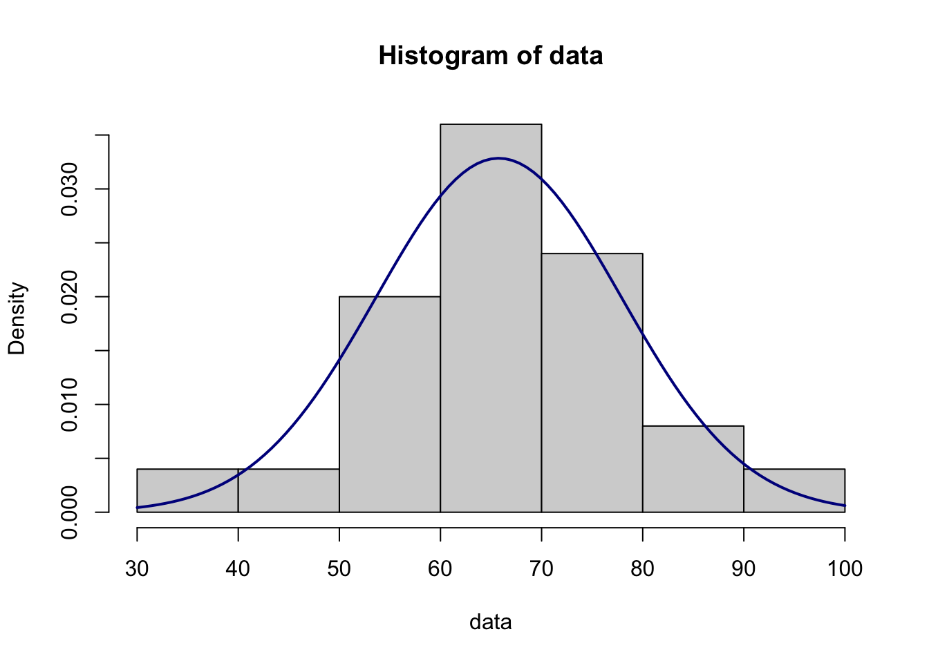

import numpy as np
import math as math
from scipy import stats
from scipy.stats import skew, kurtosis, anderson, kstest, norm

data = [76, 62, 55, 62, 56, 64, 44, 56, 94, 37, 72, 85, 72, 71, 60, 61, 64, 71, 69, 70, 64, 59, 71, 65, 84]

m = np.mean(data)

s = np.std(data, ddof=1)

skew = skew(data, bias=False)

kurt = kurtosis(data, bias=False)

IQR_to_s = stats.iqr(data) / s

within1s = np.mean(np.abs(data - m) < s)

within2s = np.mean(np.abs(data - m) < 2 * s)

within3s = np.mean(np.abs(data - m) < 3 * s)

SW_res = stats.shapiro(data)

JB_res = stats.jarque_bera(data)

AD_res = stats.anderson(data)

AD2 = AD_res[0]*(1 + (.75/50) + 2.25/(50**2))

if AD2 >= .6:
    AD_p = math.exp(1.2937 - 5.709*AD2 - .0186*(AD2**2))
elif AD2 >=.34:
    AD_p = math.exp(.9177 - 4.279*AD2 - 1.38*(AD2**2))
elif AD2 >.2:
    AD_p = 1 - math.exp(-8.318 + 42.796*AD2 - 59.938*(AD2**2))
else:
    AD_p = 1 - math.exp(-13.436 + 101.14*AD2 - 223.73*(AD2**2))

KS_res = kstest(data, norm(loc=np.mean(data), scale=np.std(data)).cdf)

results = {
    'Mean': m,
    'St. deviation': s,
    'Sample size': len(data),
    'Skewness (~=0?)': skew,
    'Excess kurtosis (~=0?)': kurt,
    'IQR/s (~=1.3?)': IQR_to_s,
    '68% rule': within1s * 100,
    '95% rule': within2s * 100,
    '100% rule': within3s * 100,
    'Test stat. - SW test': SW_res[0],
    'P-value - SW test': SW_res[1],
    'Test stat. - JB test': JB_res[0],
    'P-value - JB test': JB_res[1],
    'Test stat. - AD test': AD_res[0],
    'P-value - AD test': AD_p,
    'Test stat. - KS test': KS_res[0],
    'P-value - KS test': KS_res[1]
}


for key, value in results.items():
    print(f"{key}: {value}")
## Mean: 65.76
## St. deviation: 12.145918381634768
## Sample size: 25
## Skewness (~=0?): -0.002892878582795321
## Excess kurtosis (~=0?): 1.121315636006976
## IQR/s (~=1.3?): 0.9056540357320815
## 68% rule: 80.0
## 95% rule: 92.0
## 100% rule: 100.0
## Test stat. - SW test: 0.9648927450180054
## P-value - SW test: 0.5202044248580933
## Test stat. - JB test: 0.47957863171421605
## P-value - JB test: 0.7867936085428064
## Test stat. - AD test: 0.44551364110243696
## P-value - AD test: 0.27208274566708046
## Test stat. - KS test: 0.14001867878746022
## P-value - KS test: 0.6601736174333425import matplotlib.pyplot as plt
# Histogram
plt.hist(data, density=True)
xmin, xmax = plt.xlim()
x = np.linspace(xmin, xmax, 100)
p = stats.norm.pdf(x, m, s)
plt.plot(x, p, 'k', linewidth=2, color="darkblue")
plt.show()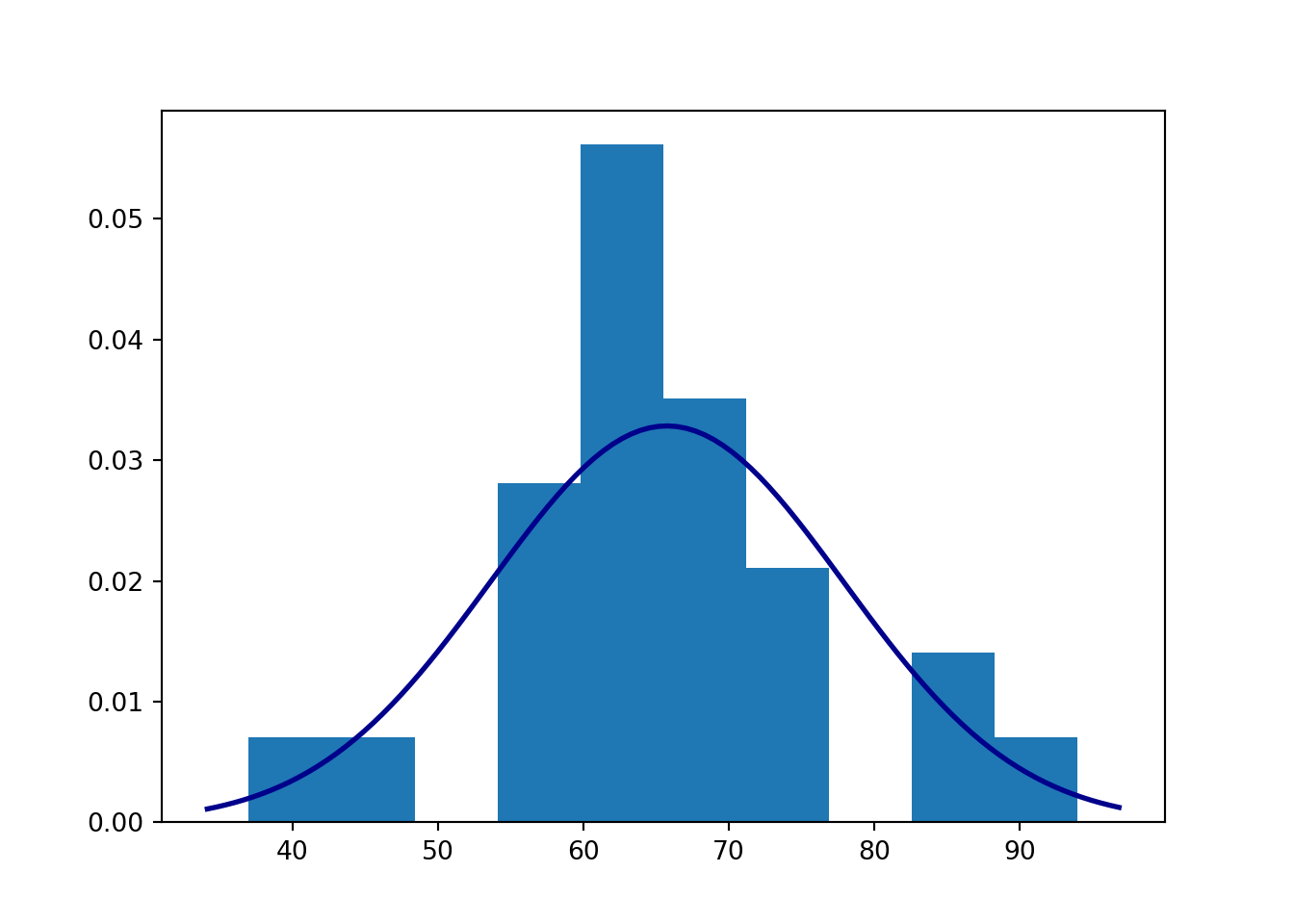
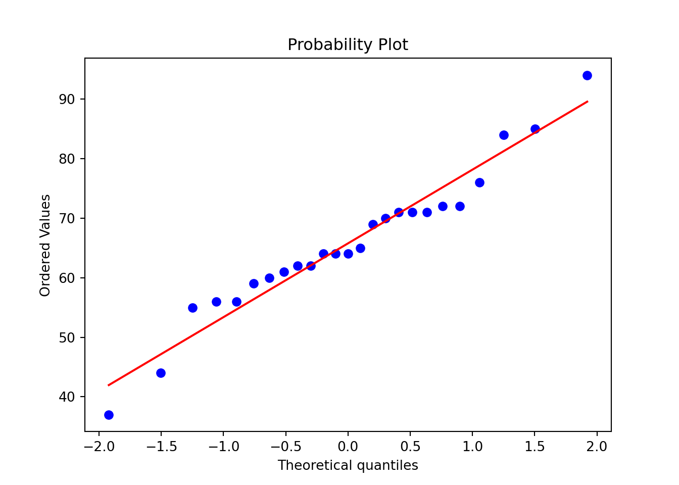
C.8.3 Correlation
Correlation — Google spreadsheet
Correlation — Excel template
#data:
x <- c(4, 8, 6, 5, 3, 8, 6, 5, 5, 6, 3, 3, 3, 7, 3, 6, 4, 4, 8, 7)
y <- c(4, 6, 8, 3, 4, 6, 5, 8, 1, 4, 4, 3, 1, 6, 7, 5, 4, 4, 9, 5)
#test and confidence interval:
cor.test(x, y, alternative = "two.sided", conf.level = 0.95)
##
## Pearson's product-moment correlation
##
## data: x and y
## t = 2.56, df = 18, p-value = 0.01968
## alternative hypothesis: true correlation is not equal to 0
## 95 percent confidence interval:
## 0.09607185 0.78067292
## sample estimates:
## cor
## 0.5166288import scipy.stats as stats
import numpy as np
x = [4, 8, 6, 5, 3, 8, 6, 5, 5, 6, 3, 3, 3, 7, 3, 6, 4, 4, 8, 7]
y = [4, 6, 8, 3, 4, 6, 5, 8, 1, 4, 4, 3, 1, 6, 7, 5, 4, 4, 9, 5]
correlation_test = stats.pearsonr(x, y)
# Confidence interval:
ci_tmp = stats.norm.interval(0.95,
loc=0.5*math.log((1+correlation_test[0])/(1-correlation_test[0])),
scale=1/((len(x)-3)**0.5))
confidence_interval = (np.exp(2*np.array(ci_tmp))-1)/(np.exp(2*np.array(ci_tmp))+1)
print('Test:\n\n', correlation_test, '\n\n Confidence interval: \n\n', confidence_interval)## Test:
##
## PearsonRResult(statistic=0.5166287822129882, pvalue=0.01968490591016886)
##
## Confidence interval:
##
## [0.09607185 0.78067292]