15 Hypothesis testing — one proportion
15.1 Single proportion test based on the \(z\) statistic
- In a single proportion test, the null hypothesis states that the proportion in the population from which the sample is drawn equals \(p_0\) (i.e., it takes a specific value stated in the hypothesis):
\[ H_0: p = p_0 \] 2. The alternative hypothesis must be chosen from three options. in a two-sided test:
\[H_A: p \ne p_0\] In a left-sided test: \[H_A: p < p_0 \]
In a right-sided test:
\[H_A: p > p_0 \]
- The test statistic (\(z\)):
\[\begin{equation} z= \frac{\hat{p}-p_0}{\sqrt{p_0 q_0/n}} \tag{15.1} \end{equation}\]
where \(\hat{p}\) is the sample proportion, \(p_0\) is the assumed proportion in the population under the null hypothesis (\(p\)), \(q_0=1-p_0\), and \(n\) is the sample size.
The rejection region depends on the alternative hypothesis. The rules for determining it are analogous to those in the \(z\) test for the mean (14.8).
As always, the sample should be random and drawn from the studied population. To use the test, the minimum sample size conditions should be met: \(np_0 \geq 15\) and \(nq_0 \geq 15\) (sometimes this requirement is lowered from 15 to 5).
15.2 p-value
P-value7 (test probability) is the probability of obtaining a test statistic at least as extreme as the one observed, assuming that the null hypothesis is true. for example, if the test statistic \(z\) in a specific sample is 2, then for a two-sided test p-value is \(\mathbb{P}(|Z|\geqslant2) \approx0,0455\), for a right-sided test \(\mathbb{P}(Z\geqslant2)\approx0,0228\), and for a left-sided test \(\mathbb{P}(Z\leqslant2) \approx 0,9772\).
Therefore, to calculate p-value, one needs to know the form of the alternative hypothesis, the distribution of the test statistic, and the value of the test statistic in a specific sample.
Very often, the p-value is calculated by a computer program (usually a statistical package). It can then be used to decide whether to reject \(H_0\) based on the results of a statistical test.
The test statistic falls within the rejection region if and only if the p-value is smaller than \(\alpha\). Instead of looking at the critical value and checking whether the test statistic falls into the rejection region, we can look at the p-value and check whether it is smaller than \(\alpha\). If p<\(\alpha\), we reject the null hypothesis.
This is convenient because statistical tests come in many forms, each with its own test statistics and critical regions, yet the approach to the p-value remains consistent. Thus, the p-value serves as a unifying principle across statistical tests.
It is important to note that p-value is not the probability that the null hypothesis is true or false. To understand this, it is worth reconsidering exercise 5.11.
15.3 Power of a test
Power of a statistical test is the (conditional) probability of not making a type II error. More precisely, test power is the probability of rejecting the null hypothesis if a specific point alternative hypothesis is true.
Type ii error is denoted by \(\beta\), hence test power is most often denoted as \(1-\beta\).
To determine the power of a given statistical test, one must:
specify the sample size (n), as power depends on the amount of data available;
define the significance level \(\alpha\), which sets the threshold for rejecting the null hypothesis.
determine the rejection region, specifying whether the test is one-sided or two-sided,
choose a specific point alternative hypothesis (such as "true proportion value" \(H_1: p = 0{,}5\)), since power is calculated for a particular alternative.
Generally, in hypothesis testing, the alternative hypothesis (denoted in this script by \(H_A\)) is a range/interval. However, test power is determined for one specific "point" value.
15.4 Links
Test power – illustration using the example of testing 2 means: https://rpsychologist.com/d3/nhst/
Test power – illustration using the example of testing 1 proportion: https://istats.shinyapps.io/power/
15.5 Templates
Spreadsheets
Tests for 1 population (mean and proportion) — Google spreadsheet
Tests for 1 population (mean and proportion) — Excel template
R code
# Test for 1 proportion
# Sample size:
n <- 200
# Number of favourable observations:
x <- 90
# Sample proportion:
p <- x/n
# Significance level:
alpha <- 0.1
# Null proportion value:
p0 <- 0.5
# Alternative (sign): "<"; ">"; "<>"; "≠"
alt <- "≠"

alttext <- if(alt==">") {"greater"} else if(alt=="<") {"less"} else {"two.sided"}

test <- prop.test(x, n, p0, alternative=alttext, correct=FALSE)
test_z <- unname(sign(test$estimate-test$null.value)*sqrt(test$statistic))
crit_z <- if(test$alternative=="less") {qnorm(alpha)} else if(test$alternative=="greater") {qnorm(1-alpha)} else {qnorm(1-alpha/2)}

print(c('Sample proportion' = test$estimate,
        'Sample size' = n,
        'Null hypothesis' = paste0('p = ', test$null.value),
        'Alternative hypothesis' = paste0('p ', alt, ' ', test$null.value),
        'Test stat. z' = test_z,
        'Test. stat. chi^2' = unname(test$statistic),
        'Critical value (z)' = crit_z,
        'P-value' = test$p.value
))
## Sample proportion.p Sample size Null hypothesis Alternative hypothesis Test stat. z
## "0.45" "200" "p = 0.5" "p ≠ 0.5" "-1.4142135623731"
## Test. stat. chi^2 Critical value (z) P-value
## "2" "1.64485362695147" "0.157299207050284"Python code
# Test for 1 proportion
from statsmodels.stats.proportion import proportions_ztest

# Sample size:
n = 200
# Number of favourable observations:
x = 90
# Sample proportion:
p = x/n
# Significance level:
alpha = 0.1
# Null proportion value:
p0 = 0.5
# Alternative hypothesis (sign): "<"; ">"; "<>"; "≠"
alt = "≠"

if alt == ">":
    alttext = "larger"
elif alt == "<":
    alttext = "smaller"
else:
    alttext = "two-sided"

test_result = proportions_ztest(count = x, nobs = n, value = p0, alternative = alttext, prop_var=p0)

print("Test statistic (z):", test_result[0], "\np-value:", test_result[1])
## Test statistic (z): -1.4142135623730947
## p-value: 0.1572992070502853315.6 Exercises
Exercise 15.1 Mr. Onur Güntürkün, in an article published in Nature in 2003 (Güntürkün 2003), described that he observed couples aged 13–70 kissing in public places (airports, train stations, parks, and beaches) in the USA, Turkey, and Germany. He recorded which way they tilted their heads while kissing. Out of 124 couples he observed, 80 tilted their heads to the right, while the remaining ones tilted their heads to the left.
Based on this, can we conclude that the probability of a randomly chosen kissing couple tilting their head to the right is significantly greater than 0.5? What assumptions must be met to use the test in this case?
Exercise 15.2 A geopolitical analyst claims that 75% of his predictions come true. A fact-checker argues that this percentage is lower than 60%. To verify this, the fact-checker reviewed 60 predictions made by the analyst and found that 28 of them could be considered accurate.
Assuming that these 60 predictions form a random sample, conduct an appropriate test to determine whether the data suggests that the prediction accuracy is significantly lower than 75%. What about lower than 60%?
Exercise 15.3 In his thesis, Mr. Łukasz investigated whether investing in selected NASDAQ stocks based on the white marubozu candlestick pattern could be profitable. This pattern appeared 107 times in the analyzed period, and in 60 cases, it resulted in a profit (i.e., buying stocks after the pattern appeared and selling them after 10 days would have been profitable).
Assume that a random investment in these stocks during the studied period would yield a profit in 51% of cases. Conduct the appropriate test, assuming a significance level of \(\alpha = 0.1\).
Exercise 15.4 (Agresti and Kateri 2021) In a certain experiment, 116 people participated. For each of them, astrologers prepared a horoscope based on their birth date. Then, for each horoscope, astrologers were presented with a questionnaire filled out by that person and two other questionnaires.
The astrologer's task was to guess which of the three questionnaires was filled out by the person for whom the horoscope was prepared. The astrologers correctly identified the person in 40 out of 116 cases.
Can we reject the null hypothesis stating that astrologers were guessing randomly? Assume \(\alpha = 0.05\).
What was the test's power, assuming that the point alternative hypothesis from the National Council for Geocosmic Research (an organization of astrologers) was that astrologers would correctly identify at least half of the cases?
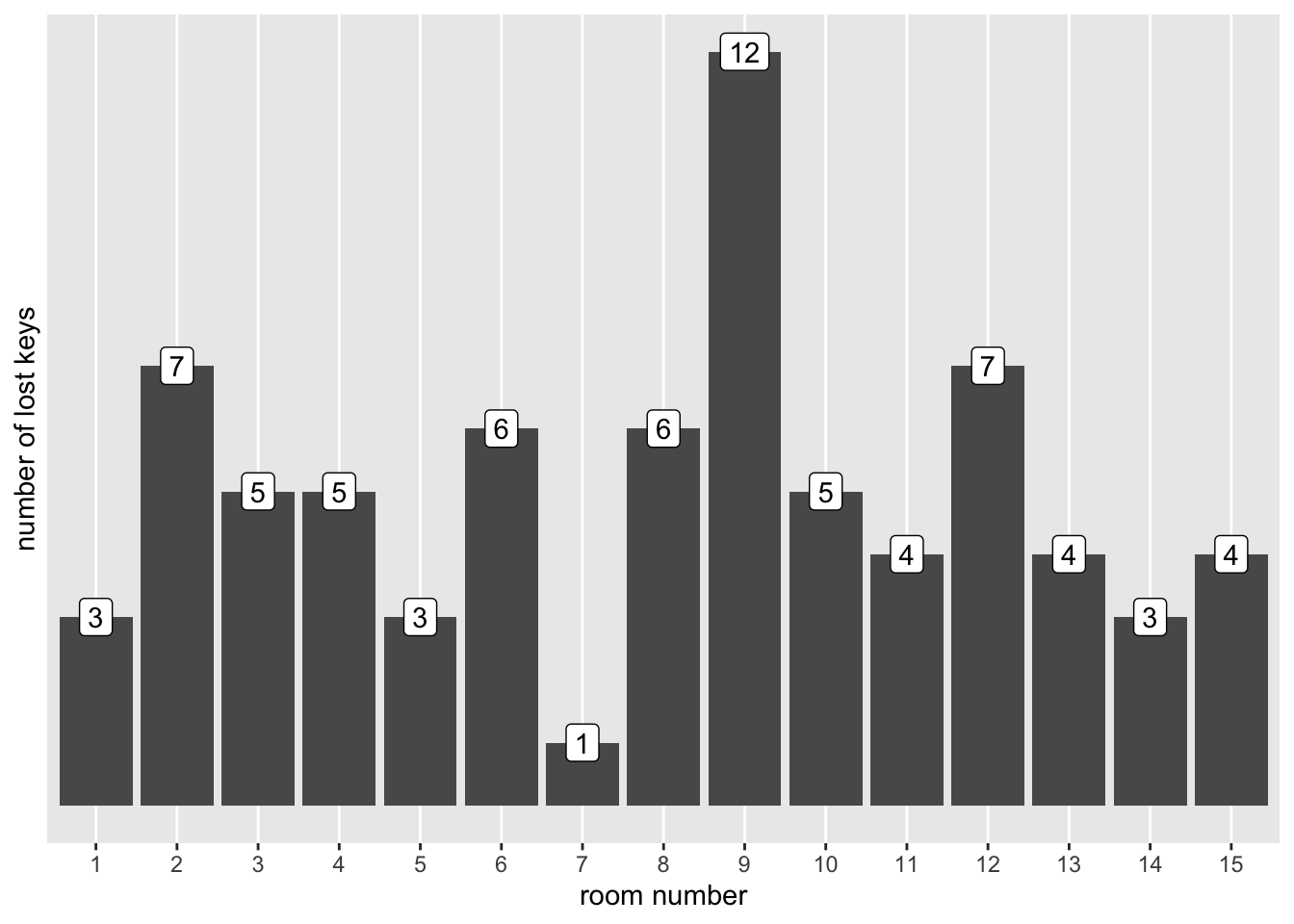
Exercise 15.5 In the short story "Nine" (part of the novel "Flights"), Olga Tokarczuk describes a hotel where key number nine was lost more often than other keys.
Assume we obtained data from this hotel. It has 15 rooms, and the total number of lost keys since the hotel was established is 75. The distribution of lost keys per room is shown in the following graph.
Test whether the proportion of “nines” among lost keys is greater than the proportion expected under a uniform distribution (1/15).
Note: The wording of this hypothesis may constitute a misuse of a statistical test. Why is this the case? What would be a more appropriate hypothesis? The suitable statistical test for this scenario will be introduced in a later chapter.
Exercise 15.6 (Agresti, Franklin, and Klingenberg 2016) SA fast-food chain wants to compare two methods of promoting a new turkey burger. One method involves using in-store coupons, while the other involves displaying posters outside the store.
Before the promotion, the marketing department paired 50 stores, ensuring each pair had comparable sales volume and similar customer demographics. A random draw determined which store in each pair would use coupons.
After one month, the sales growth of the turkey burger was compared within each store pair. In 28 cases, the store using coupons showed higher sales growth, while in 22 cases, the store using posters had a greater increase.
Is this strong enough evidence to favor the coupon-based approach, or could this result be due to chance?
Literature
Note that p-value is another instance where we use the letter p as a symbol. We have already had \(\mathbb{P}\) as a probability function of an event (4), \(\textbf{p}\) as a probability mass function of a discrete variable (7.1), \(p\) as the probability of success in a single trial in the binomial distribution (??), \(p\) as the population proportion, and \(\hat{p}\) as the sample proportion (10). now we encounter p once again, perhaps for the last time.↩︎