Estimating Demand

Introduction

In the early 1970s, San Francisco was completing a huge new infrastructure project, the Bay Area Rapid Transit (BART) system. The project initially cost $1.6 billion and included tunneling under the San Francisco Bay. Policy makers were obviously interested in determining how many people would use the new system once it was built. But that is a problem. How do you predict the demand for a product that does not exist?

One solution is to ask people. A survey was conducted of people who were likely to use the new transport system. The survey asked detailed questions about their current mode of transport and asked them whether they would use the new system. The concern is that it is hard for people to predict how they would use something that does not exist. Berkeley econometrician, Dan McFadden, suggested an alternative approach. Instead of asking people to predict what they would do, McFadden suggested using information on what people actually do do, then use economic theory to predict what they would do.

McFadden argued that combining survey data with economic theory would produce more accurate estimates than the survey data alone (McFadden 1974). In the case of the BART survey, McFadden was correct. According to the survey data, 15% of respondents said that they would use BART. McFadden estimated that 6% of respondents would use BART. In fact, 6% of respondents actually did use BART.¹ Survey data is valuable, but people give more accurate answers to some questions than others.

The first part of the book discussed how exogenous variation is needed to use observed data to predict policy outcomes. Chapters 1 and 2 assume that observed variation in exposure to a policy is determined independently of unobserved characteristics. Chapters 3 and 4 relaxed this assumption but allowed economic theory to be used in estimating the impact of the policy. This part of the book extends the idea of using economic theory. This chapter introduces the idea of using revealed preference.

Today, the ideas that McFadden developed for analyzing the value of BART are used across economics, antitrust, marketing, statistics and machine learning. At the Federal Trade Commission and the Department of Justice, economists use these techniques to determine whether a merger between ice cream manufacturers, or cigarette manufacturers, or supermarkets, or hospitals, will lead to higher prices.

When Google changed the way it displayed search results, user traffic moved away from Google’s competitors. Such actions by a dominant firm like Google could lead to antitrust actions unless the changes also made users better off. By combining economic theory and data on the behavior of Google’s users, we can determine whether Google’s changes were pro or anti-competitive. According to the FTC’s statement on the Google investigation, analysis of Google’s click through data by staff economists showed that consumers benefited from the changes that Google made. This, and other evidence, led the FTC to end its investigation of Google’s “search bias” practice with a 5-0 vote.²

The chapter begins with basic economic assumption of demand estimation, revealed preference. It takes a detour to discuss the maximum likelihood algorithm. It returns with Daniel McFadden’s model of demand. The chapter introduces the logit and probit estimators, and uses them to determine whether consumers in small US cities value rail as much as their big city neighbors.

Revealed Preference

McFadden’s analysis, and demand analysis more generally, relies on the following assumption.

(Revealed Preference) If there are two choices, \(A\) and \(B\), and we observe a person choose \(A\), then her utility from \(A\) is greater than her utility from \(B\).

Assumption 1

The Assumption 1 states that if we observe someone choose product \(A\) when product \(B\) was available, then that someone prefers product \(A\) to product \(B\). The assumption allows the researcher to infer unobserved characteristics from observed actions. It is also a fundamental assumption of microeconomics. Do you think it is a reasonable assumption to make about economic behavior?

The section uses simulated data to illustrate how revealed preference is used to estimate consumer preferences.

Modeling Demand

Consider a data set where a large number of individuals are observed purchasing either product \(A\) or product \(B\) at various prices for the two products. Each individual will have some unobserved characteristic \(u\), that we can call utility. We make two important assumptions about the individuals. First, their value for purchasing one of the two products is \(u_{Ai} - p_A\). It is equal to their unobserved utility for product \(A\) minus the price of product \(A\). Their utility is **linear in money}.³ Second, if we observe person \(i\) purchase \(A\) at price \(p_A\) then we know that the following inequality holds.

\[ \begin{array}{l} u_{Ai} - p_A > u_{Bi} - p_B\\ \mbox{or }\\ u_{Ai} - u_{Bi} > p_A - p_B \end{array} \tag{1}\]

Person \(i\) purchases good \(A\) if and only if her relative utility for \(A\) is greater than the relative price of \(A\).

We usually make a transformation to normalize everything relative to one of the available products. That is, all prices and demand are made relative to one of the available products. Here we will **normalize} to product \(B\). So \(p = p_A - p_B\) and \(u_i = u_{Ai} - u_{Bi}\). Prices and utility are net of prices and utility for product \(B\).

In addition, we often observe the data at the market level rather than the individual level. That is, we see the fraction of individuals that purchase \(A\). Below this fraction is denoted \(s\). It is the share of individuals that purchase \(A\).

Simulating Demand

The simulated data illustrates the power of the revealed preference assumption. Consider the following distribution of an unobserved term. The unobserved term is drawn from a normal distribution with a mean of 1 and a variance of 9 (\(u \sim \mathcal{N}(1, 9)\)). Let’s assume that we have data on 1,000 people and each of them is described by this \(u\) characteristic.

set.seed(123456789)
N <- 1000
u <- sort(rnorm(N, mean=1, sd=3))

Can we uncover this distribution from observed behavior of the individuals in our simulated data? Can we use the revealed preference assumption to uncover the unobserved term (\(u\))?

p <- 2
mean(u - p > 0) # estimated probability

[1] 0.386

1 - pnorm(p, mean=1, sd=3) # true probability

[1] 0.3694413

If \(p = 2\), then the share of people who purchase \(A\) is 39%, which is approximately equal to the probability that \(u\) is greater than 2. Combining the revealed preference assumption with the observed data allows us to uncover the fraction of simulated individuals whose value for the unobserved characteristic is greater than 2.

Revealing Demand

If we are able to observe a large number of prices, then we can use revealed preference to estimate the whole distribution of the unobserved utility. At each price, the share of individuals purchasing product \(A\) is calculated. If we observe enough prices then we can use the observed shares at each price to plot out the demand curve.

p <- runif(9,min=-10,max=10)
# 9 points between -10, 10.
s <- matrix(NA,length(p),1)  # share of market buying A.
for (i in 1:length(p)) {
  s[i,1] <- mean(u - p[i] > 0)
  #print(i)
}

plot(1-ecdf(u)(u),u, type="l",lwd=3,lty=1,col=1, 
     xlab="s", ylab="p", xlim=c(0,1))
# ecdf(a)(a) presents the estimated probabilities of a.
lines(sort(s),p[order(s)], type="l", lwd=3,lty=2)
legend("bottomleft",c("True","Est"),lwd=3,lty=c(1:2))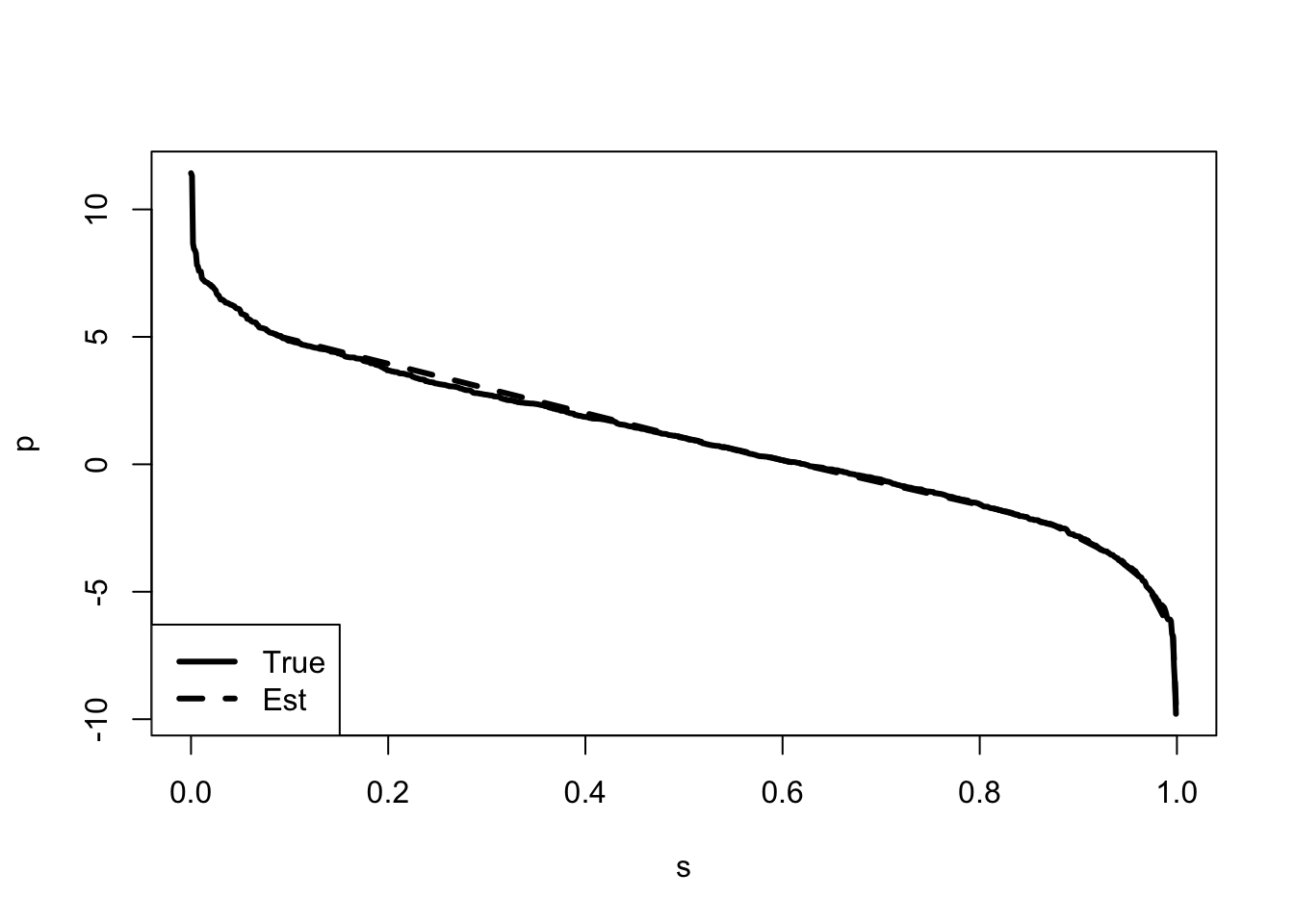

Figure 1: Plot of survival function and estimated demand.

The Figure 1 presents the estimated demand curve.

Discrete Choice

Demand estimation often involves outcomes with discrete values. In McFadden’s original problem, we observe one of three choices, car, bus, or train. OLS tends not to work very well when the outcome of interest is discrete or limited in some manner. Given this, it may be preferable to use a discrete choice model such as a logit or probit.⁴

The section uses simulated data to illustrate issues with estimating the discrete choice model.

Simple Discrete Choice Model

Consider the following discrete model. There is some latent (hidden) value of the outcome (\(y_i^*\)), where if this value is large enough we observe \(y_i = 1\).

\[ \begin{array}{l} y_i^* = a + b x_i + \upsilon_i\\ \\ y_i = \left \{\begin{array}{l} 1 \mbox{ if } y_i^* \ge 0\\ 0 \mbox{ if } y_i^* < 0 \end{array} \right. \end{array} \tag{2}\]

We can think of \(y_i^*\) as representing utility and \(y_i\) as representing observed demand.

Simulating Discrete Choice

In the simulated data there is a latent variable (\(y^*\)) that is determined by a model similar to the one presented in Chapter 1.⁵ Here, however, we do not observe \(y^*\). We observe \(y\) which only has values 0 or 1.

set.seed(123456789)
N <- 100
a <- 2
b <- -3
u <- rnorm(N)
x <- runif(N)
ystar <- a + b*x + u
y <- ystar > 0
lm1 <- lm(y ~ x)

Figure 2: Plot of \(x\) and \(y\) with the relationship between \(y^*\) and \(x\) represented by the solid line. The estimated relationship is represented by the dashed line.

The Figure 2 shows that the estimated relationship differs substantially from the true distribution. The figure illustrates how OLS fails to accurately estimate the parameters of the model. In order to correctly estimate the relationship we need to know the distribution of the unobserved term.

Modeling Discrete Choice

We can write out the model using matrix notation.

\[ \begin{array}{l} y_i^* = \mathbf{X}_i' \beta + \upsilon_i\\ \\ y_i = \left \{\begin{array}{l} 1 \mbox{ if } y_i^* \ge 0\\ 0 \mbox{ if } y_i^* < 0 \end{array} \right . \end{array} \tag{3}\]

where \(\mathbf{X}_i\) is a vector of observed characteristics of individual \(i\), \(\beta\) is a vector that maps from the observed characteristics to the latent outcome, \(y_i^*\), and \(\upsilon_i\) is the unobserved term. The observed outcome, \(y_i\) is equal to 1 if the latent variable is greater than 0 and it is 0 if the latent variable is less than 0.

The probability of observing one of the outcomes (\(y_i = 1\)) is as follows.

\[ \begin{array}{l} \Pr(y_i = 1 | \mathbf{X}_i) & = \Pr(y_i^* > 0)\\ & = \Pr(\mathbf{X}_i' \beta + \upsilon_i > 0)\\ & = \Pr(\upsilon_i > - \mathbf{X}_i' \beta)\\ & = 1 - F(- \mathbf{X}_i' \beta) \end{array} \tag{4}\]

where \(F\) represents the probability distribution function of the unobserved characteristic.

If we know \(\beta\), we can determine the distribution of the unobserved term with variation in the \(X\)s. That is, we can determine \(F\). This is exactly what we did in the previous section. In that section, \(\beta = 1\) and variation in the price (the \(X\)s) determines the probability distribution of \(u\). However, we do not know \(\beta\). In fact, \(\beta\) is generally the policy parameter we want to estimate. We cannot identify both \(\beta\) and \(F\) without making some restriction on one or the other.

The standard solution is to assume we know the true distribution of the unobserved term (\(F\)). In particular, a standard assumption is to assume that \(F\) is standard normal. Thus, we can write the probability of observing the outcome \(y_i = 1\) conditional on the observed \(X\)s.

\[ \Pr(y_i = 1 | \mathbf{X}_i) = 1 - \Phi(-\mathbf{X}_i' \beta) \tag{5}\]

where \(\Phi\) is standard notation for the standard normal distribution function.

Maximum Likelihood

The standard algorithm for estimating discrete choice models is maximum likelihood. The maximum likelihood algorithm generally requires some assumption about the distribution of the error term. However, as seen above, we are generally making such an assumption anyway.

This section takes a detour to illustrate how the maximum likelihood algorithm works.

Binomial Likelihood

Consider the problem of determining whether a coin is “fair.” That is, whether the coin has an equal probability of Heads or Tails, when tossed. If the coin is weighted then it may not be fair. It may have a greater probability of landing on Tails than on Heads. The code simulates an unfair coin. The observed probability of a head is 34 of 100.

set.seed(123456789)
N <- 100
p <- 0.367 # the true probability of Head.
Head <- runif(N) < p
mean(Head) # the observed frequency of Head.

[1] 0.34

What is the likelihood that this data was generated by a fair coin? It is the probability of observing 34 Heads and 66 Tails given that the true probability of a Head is 0.5.

What is the probability of observing 1 Head given the true probability is 0.5? It is just the probability of Heads, which is 0.5.

\[ \Pr(\mathrm{Head} | p = 0.5) = 0.5 \tag{6}\]

What is the probability of observing three Heads and zero Tails? If the coin tosses are independent of each other, then it is the probability of each Head, all multiplied together.⁶

\[ \Pr(\{\mathrm{Head}, \mathrm{Head}, \mathrm{Head}\} | p = 0.5) = 0.5 \times 0.5 \times 0.5 = 0.5^3 \tag{7}\]

How about three Heads and two Tails?

\[ \Pr(\{3\mathrm{ Heads}, 2\mathrm{ Tails}\}) = 0.5^3 0.5^2 \tag{8}\]

Actually, it isn’t. This is the probability of observing 3 Heads and *then} 2 Tails. But it could have been 1 Head, 2 Tails, 2 Heads or 1 Tail, 1 Head, 1 Tail, 2 Heads etc., etc. There are a number of different combinations of results that have 3 Heads and 2 Tails. In this case there are \(\frac{5!}{3!2!} = 10\) different permutations, where 5! means 5 factorial or 5 multiplied by 4 multiplied by 3 multiplied by 2 multiplied by 1.

In R we can use factorial() to do the calculation.

factorial(5)/(factorial(3)*factorial(2))

[1] 10

What is the likelihood of observing 34 Heads and 66 Tails? If the true probability is 0.5, the likelihood is given by the binomial function.

\[ \Pr(\{34 H, 66 T\} | p = 0.5) = \frac{100!}{34! 66!} 0.5^{34} 0.5^{66} \tag{9}\]

What is the likelihood of observing \(\hat{p}\) Heads in \(N\) trials? Given a true likelihood of \(p\), it is given by the binomial function.

\[ \Pr(\hat{p} | p, N) = \frac{N!}{(\hat{p} N)! ((1 - \hat{p}) N)!} p^{\hat{p} N} (1 - p)^{(1 - \hat{p})N} \tag{10}\]

In R we can use the choose() function to calculate the coefficient for the binomial function.

choose(100, 34)*(0.5^100)

[1] 0.0004581053

The likelihood that the coin is fair seems small.

What is the most likely true probability? One method uses the analogy principle. If we want to know the true probability then we use the analogy in the sample. The best estimate of the true probability is the observed frequency of Heads in the sample (Manski 1990).⁷ It is 34/100. Note that this is not equal to the true probability of 0.367, but it is pretty close.

Alternatively, find the probability that maximizes the likelihood. What is the true probability \(p\) that has the highest likelihood of generating the observed data? It is the true probability that maximizes the following problem.

\[ \begin{array}{l} \max_{p \in [0, 1]} \frac{N!}{(\hat{p} N)! ((1 - \hat{p}) N)!} p^{\hat{p} N} (1 - p)^{(1 - \hat{p})N} \end{array} \tag{11}\]

It is not a great idea to ask a computer to solve the problem as written. The issue is that these numbers can be very very small. Computers have a tendency to change very small numbers into other, totally different, small numbers. This can lead to errors.

Find the probability that maximizes the log likelihood.

\[ \begin{array}{l} \max_{p \in [0, 1]} \log(N!) - log((\hat{p} N)!)- \log((1 - \hat{p}) N)!)\\ + \hat{p} N \log(p) + (1 - \hat{p})N \log(1 - p) \end{array} \tag{12}\]

The solution to this problem is identical to the solution to the original problem.⁸

Binomial Likelihood in R

The Equation 12 provides pseudo-code for a simple optimizer in R. We can use the optimize() function to find the minimum value in an interval.⁹ Note also that the function being optimized dropped the coefficient of the binomial function. Again, this is fine because the optimum does not change.

ll_function <- function(p, N, p_hat) {
  return(-((p_hat*N)*log(p) + (1 - p_hat)*N*log(1-p)))
  # Note the negative sign as optimize is a minimizer.
}
optimize(f = ll_function, interval=c(0,1), N = 100, p_hat=0.34)

$minimum
[1] 0.3399919

$objective
[1] 64.10355

The maximum likelihood estimate is 0.339, which is fairly close to the analog estimate of 0.34. Figure 3 shows that the likelihood function is relatively flat around the true value. The implication is that the difference in the likelihood between the true value and the estimated value is quite small.

p <- c(1:1000)/1000
log_lik <- sapply(p, function(x) lchoose(100,34) + 34*log(x) +
                 66*log(1-x))
# sapply is a quick way for R to apply a function to a set
# note that we have defined the function on the fly.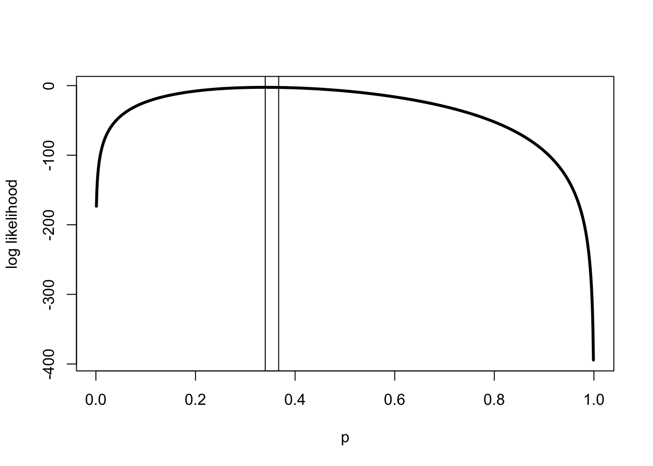

Figure 3: Plot of log likelihood for a sample with 34 Heads out of 100. Lines at the analog estimate of 0.34 and the true value of 0.367.

OLS with Maximum Likelihood

We can use maximum likelihood to estimate OLS. Chapter 1 presented the standard algorithms for estimating OLS. It points out that with an additional assumption, the maximum likelihood algorithm could also be used instead.

Assume we have data generated by the following linear model.

\[ y_i = \mathbf{X}_i' \beta + \upsilon_i \tag{13}\]

where \(y_i\) is the outcome of interest, \(\mathbf{X}_i\) is a vector representing observed characteristics of individual \(i\), and \(\upsilon_i\) represents the unobserved characteristics of individual \(i\). As is normally the case, we are interested in estimating \(\beta\).

We can use maximum likelihood to estimate parameters of this model. However, we must assume that \(\upsilon_i\) has a particular distribution. A standard assumption is that \(\upsilon_i \sim \mathcal{N}(0, \sigma^2)\). That is, we assume the unobserved characteristic is normally distributed. Note that we don’t know the parameter, \(\sigma\).

We can determine the likelihood of observing the data by first rearranging Equation 13.

\[ \upsilon_i = y_i - \mathbf{X}_i' \beta \tag{14}\]

The probability of observing the outcome is as follows.

\[ \begin{array}{l} f(\upsilon_i | y_i, \mathbf{X}_i) = \frac{1}{\sigma} \phi \left(\frac{\upsilon_i - 0}{\sigma} \right)\\ = \frac{1}{\sigma} \phi (z_i) \end{array} \tag{15}\]

where

\[ z_i = \frac{y_i - \mathbf{X}_i'\beta}{\sigma} \tag{16}\]

and \(\phi\) is the standard normal density.

Note in R, it is necessary to use the standard normal distribution function.¹⁰ To use this function we need to normalize the random variable by taking away the mean of the unobserved term, which is zero, and by dividing by the standard deviation of the unobserved term (\(\sigma\)). The standard notation for the normalized variable is \(z\), but don’t confuse this with our notation for an instrumental variable. We also need to remember that this is the density, a derivative of the probability distribution function. Therefore, we need to adjust the density formula by dividing it by the standard deviation of the distribution of the unobserved characteristic (\(\sigma\)).

Therefore, the likelihood of observing the data is given by the following product.

\[ L(\{y,\mathbf{X}\} | \{\beta, \sigma\}) = \prod_{i=1}^N \left (\frac{1}{\sigma} \phi\left(\frac{y_i - \mathbf{X}_i'\beta}{\sigma} \right) \right ) \tag{17}\]

The sample size is \(N\) and \(\prod_{i=1}^N\) is notation for multiply all the items denoted 1 to \(N\) together.¹¹

We can find the maximum likelihood estimates of \(\beta\) and \(\sigma\) by solving the following problem.

\[ \max_{\beta,\sigma} \sum_{i=1}^N \log \left(\phi\left(\frac{y_i - \mathbf{X}_i'\beta}{\sigma} \right) \right) - N \log(\sigma) \tag{18}\]

Compare this to the estimator in Chapter 1.¹²

Maximum Likelihood OLS in R

We can create a maximum likelihood estimator of the OLS model using Equation 18 as pseudo-code.

f_ols <- function(para, y, X) {
  X <- cbind(1,X)
  N <- length(y)
  J <- dim(X)[2]
  sig <- exp(para[1])
  # Note that sig must be positive.  
  # The exponential function maps
  # from any real number to positive numbers.  
  # It allows the optimize to choose any value and 
  # transforms that number into a positive value.
  beta <- para[2:(J+1)]
  z <- (y - X%*%beta)/sig 
  log_lik <- -sum(log(dnorm(z)) - log(sig))
  return(log_lik)
  # remember we are minimizing.
}

The standard optimizer in R is the function optim(). This function defaults to a Nelder-Mead which is a fairly robust algorithm.

a1 <- optim(par=c(0,2,-3),fn=f_ols,y=ystar,X=x)
# optim takes in starting values with par, then the function
# used and then values that the function needs.
# we cheat by having it start at the true values.
# sig
exp(a1$par[1])

[1] 0.9519634

# beta
a1$par[2:3]

[1]  1.832333 -2.643751

Our estimate \(\hat{\sigma}\) fairly close to the true value is 1, and \(\hat{\beta} = \{1.83,-2.64\}\) compared to true values of 2 and -3. What happens if you use different starting values?

Probit

Circling back, consider the discrete choice problem that began the chapter. If we have information about the distribution of the unobserved term, which is generally assumed, then we can find the parameters that maximize the likelihood of the model predicting the data we observe.

Consider the problem described by Equation 3. Assume the unobserved characteristic is distributed standard normal, then the likelihood of observing the data is given by the following function.

\[ L(\{y, \mathbf{X}\} | \beta) = \prod_{i = 1}^N \Phi(-\mathbf{X}_i' \beta)^{1 - y_i} (1 - \Phi(-\mathbf{X}_i' \beta))^{y_i} \tag{19}\]

The Equation 19 shows the likelihood function of observing the data we actually observe (\(\{y,\mathbf{X}\}\)) given that the true probability which is determined by \(\beta\). Note that the variance of the unobserved characteristic (\(\sigma^2\)) is not identified in the data. That is, there are an infinite number of values for \(\sigma^2\) that are consistent with the observed data. The standard solution is to set it equal to 1 (\(\sigma^2 = 1\)). Note that \(y_i\) is either 0 or 1 and also note that \(a^0 = 1\), while \(a^1 = a\). This is the binomial likelihood function (Equation 11) written in a general way with the probabilities determined by the standard normal function.

The parameter of interest, \(\beta\), can be found as the solution to the following maximization problem.

\[ \max_{\beta} \sum_{i = 1}^N (1 - y_i) \log(\Phi(-\mathbf{X}_i' \beta)) + y_i \log(\Phi(\mathbf{X}_i' \beta))) \tag{20}\]

Note that I made a slight change going from Equation 19 to Equation 20. I took advantage of the fact that the normal distribution is symmetric. This version is better for computational reasons.¹³

Probit in R

f_probit <- function(beta, y, X) {
  X <- cbind(1,X)
  Xb <- X%*%beta
  log_lik <- (1 - y)*log(pnorm(-Xb)) + y*log(pnorm(Xb))
  return(-sum(log_lik))
}

optim(par=lm1$coefficients,fn=f_probit,y=y,X=x)$par

(Intercept)           x 
   2.014153   -2.835234 

We can use Equation 20 as the basis for our own probit estimator. The probit estimates are closer to the true values of 2 and -3, although they are not particularly close to the true values. Why aren’t the estimates close to the true values?¹⁴

Generalized Linear Model

The probit is an example of a generalized linear model. The outcome vector is, \(y = f(\mathbf{X} \beta)\), where \(f\) is some function. This is a generalization of the OLS model. It has a linear index, \(\mathbf{X} \beta\), but that index sits inside a potentially non-linear function (\(f\)). The probit is an example, as is the logit model discussed below.

In R these types of functions can often be estimated with the glm() function. Like the lm() function, glm() creates an object that includes numerous results including the coefficients. The nice thing about the glm() function is that it includes a variety of different models. Unfortunately, that makes it unwieldy to use.

We can compare our probit estimates to those from the built-in R probit model using glm().

glm(y ~ x, family = binomial(link="probit"))$coefficients

(Intercept)           x 
   2.014345   -2.835369 

The results are about the same. The two models are solved using different algorithms. The glm() uses an algorithm called iterative weighted least squares rather than maximum likelihood.

McFadden’s Random Utility Model

In order to estimate the impact of the BART rail system, McFadden needed a model that captured current choices and predicted demand for a product that didn’t exist.

The section presents McFadden’s model, the probit, and logit estimators and simulation results.

Model of Demand

In McFadden’s model, person \(i\)’s utility over choice \(j\) is the following random function.

\[ U_{ij} = \mathbf{X}_{ij}' \beta + \upsilon_{ij} \tag{21}\]

Person \(i\)’s utility is a function of observable characteristics of both person \(i\) and the choice \(j\) represented in Equation 21 by the matrix \(\mathbf{X}\). In the case of the BART survey, these are things like the person’s income and the cost of commuting by car. These observed characteristics are mapped into utility by person \(i\)’s preferences, represented by the \(\beta\) vector. Lastly, there are unobserved characteristics of person \(i\) and choice \(j\) that also determine the person’s value for the choice. These are represented by \(\upsilon_{ij}\).

To predict demand for BART from observed demand for cars and buses we need two assumptions. First, the preference weights (\(\beta\)) cannot vary with the product. Second, the choice can be described as a basket of characteristics. This style of model is often called an hedonic model. Commuting by car is represented by a set of characteristics like tolls to be paid, gasoline prices, parking, the time it takes, and car maintenance costs. Similarly, commuting by train or bus depends on the ticket prices and the time it takes. Individuals weight these characteristics the same irrespective of which choice they refer to.

We can use revealed preference and observed choices to make inferences about person \(i\)’s preferences. From the revealed preference assumption we learn that the person’s utility from product \(A\) is greater than their utility from product \(B\). If we observe person \(i\) face the choice between two products \(A\) and \(B\), and we see her choose \(A\), then we learn that \(U_{iA} > U_{iB}\).

\[ \begin{array}{c} U_{iA} > U_{iB}\\ \mathbf{X}_{iA}' \beta + \upsilon_{iA} > \mathbf{X}_{iB}' \beta + \upsilon_{iB}\\ \upsilon_{iA} - \upsilon_{iB} > - (\mathbf{X}_{iA} - \mathbf{X}_{iB})' \beta \end{array} \tag{22}\]

The Equation 22 shows that if there is enough variation in the observed characteristics of the choices (\(\mathbf{X}_{iA} - \mathbf{X}_{iB}\)), we can potentially estimate the unobserved characteristics (\(\upsilon_{iA} - \upsilon_{iB}\)) and the preferences (\(\beta\)). The analysis in the first section of the chapter shows how variation in prices can allow the distribution of the unobserved characteristic to be mapped out. The \(X\)s are like the price; in fact, they may be prices. We also need to make an assumption about the distribution of the unobserved characteristics (\(\upsilon_{iA} - \upsilon_{iB}\)). Next we consider two different assumptions.

Probit and Logit Estimators

If we assume that \(\upsilon_{iA} - \upsilon_{iB}\) is distributed standard normal we can use a probit model.¹⁵

\[ \begin{array}{l} \Pr(y_i = 1 | \mathbf{X}_{iA}, \mathbf{X}_{iB}) = \Pr(\upsilon_{iA} - \upsilon_{iB} > - (\mathbf{X}_{iA} - \mathbf{X}_{iB})' \beta)\\ = \Pr(-(\upsilon_{iA} - \upsilon_{iB}) < (\mathbf{X}_{iA} - \mathbf{X}_{iB})' \beta)\\ = \Phi((\mathbf{X}_{iA} - \mathbf{X}_{iB})' \beta) \end{array} \tag{23}\]

McFadden’s original paper estimates a logit. It assumes that the unobserved characteristics are distributed extreme value type 1. This mouthful-of-a-distribution is also called Gumbel or log Weibull. The advantage of this distribution is that the difference in the unobserved terms is a logistic distribution and a logit model can be used.

The logit has some very nice properties. In particular, it is very easy to compute. This made it a valuable model in the 1970s. Even today the logit is commonly used in machine learning because of its computational properties.¹⁶ The logit assumption allows the probability of interest to have the following form.

\[ \Pr(y_i = 1 | \mathbf{X}_{iA}, \mathbf{X}_{iB}) = \frac{\exp((\mathbf{X}_{iA} - \mathbf{X}_{iB})' \beta)}{1 + \exp((\mathbf{X}_{iA} - \mathbf{X}_{iB})' \beta)} \tag{24}\]

This function is very useful. It has the property that whatever parameter you give it, it returns a number between 0 and 1, a probability.¹⁷ It is often used in optimization problems for this reason.

Simulation with Probit and Logit Estimators

Consider a simulation of the McFadden model with both the probit and logit assumption on the unobserved characteristics.

set.seed(123456789)
N <- 5000
XA <- cbind(1,matrix(runif(2*N),nrow=N))
XB <- cbind(1,matrix(runif(2*N),nrow=N))
# creates two product characteristic matrices
beta <- c(1,-2,3)

In the simulation there are 5,000 individuals choosing between two products with two observable characteristics. Note that these characteristics vary across the individuals, but the preferences of the individuals do not.

# Probit
uA <- rnorm(N)
y <- XA%*%beta - XB%*%beta + uA > 0
glm1 <- glm(y ~ I(XA - XB), family = binomial(link="probit"))
# note that I() does math inside the glm() function.

The probit model assumes that the unobserved characteristic (the relative unobserved characteristic) is distributed standard normal. The logit assumes that the unobserved characteristics are distributed extreme value type 1. Note that the function I() allows mathematical operations with in the glm() or lm() function. Here it simply takes the difference between the two matrices of observed characteristics.

# Logit
uA <- log(rweibull(N, shape = 1))  
# gumbel or extreme value type 1
uB <- log(rweibull(N, shape = 1))
y <- (XA%*%beta - XB%*%beta) + (uA - uB) > 0
glm2 <- glm(y ~ I(XA - XB), family = binomial(link="logit"))

What happens if you run OLS? Do you get the right sign? What about magnitude?

Warning: package 'modelsummary' was built under R version 4.4.1

`modelsummary` 2.0.0 now uses `tinytable` as its default table-drawing
  backend. Learn more at: https://vincentarelbundock.github.io/tinytable/

Revert to `kableExtra` for one session:

  options(modelsummary_factory_default = 'kableExtra')
  options(modelsummary_factory_latex = 'kableExtra')
  options(modelsummary_factory_html = 'kableExtra')

Silence this message forever:

  config_modelsummary(startup_message = FALSE)

Warning: package 'gt' was built under R version 4.4.1

Table 1: Probit estimate (1) and logit estimate (2).

	(1)	(2)
(Intercept)	0.010	-0.018
	(0.023)	(0.033)
I(XA - XB)2	-2.023	-1.924
	(0.068)	(0.089)
I(XA - XB)3	3.016	2.861
	(0.081)	(0.099)
Num.Obs.	5000	5000
AIC	3897.2	5367.7
BIC	3916.7	5387.3
Log.Lik.	-1945.585	-2680.873
RMSE	0.36	0.42

The Table 1 presents the probit and logit estimates. The table shows that the probit gives estimates that are very close to the true values of -2 and 3. Why is the intercept term 0 rather than the true value of 1? The estimates from the logit are also relatively close to the true values. The different error assumptions of the logit may lead to wider variation in the estimates.

Multinomial Choice

In the analysis above, individuals choose between two options. In many problems individuals have many choices. This section looks at commuters choosing between car, bus, and train. It is in these multinomial choice problems that the logit really comes into its own.

The section presents a multinomial probit, actually a bivariate probit which can be used to model the choice between three options. This model is relatively general, but the computational burden increases exponentially (possibly geometrically) in the number of choices. This is called the curse of dimensionality. One solution to this computational issue is to use an ordered probit. The book doesn’t discuss this model but the model can be very useful for certain problems.

Instead, the section considers a multinomial logit and the independence of irrelevant alternatives assumption. The assumption implies that the unobserved characteristics associated with one choice are independent of the unobserved characteristics associated with any other choice. This assumption allows the logit model to handle very large choice problems. It also allows the model to handle predictions about new choices that are not in the observed data, such as the BART rail system. However, it is a strong restriction on preferences.

The section illustrates these methods with simulated data.

Multinomial Choice Model

Consider the full model of choice over three potential modes of transportation. In the model each person \(i\) has utility for each of the three choices. Note that as before, \(\beta\) is the same for each choice. It is the observed characteristics of the choices and the unobserved characteristics that change between choices.

\[ \begin{array}{l} U_{iC} = \mathbf{X}_{iC}' \beta + \upsilon_{iC}\\ U_{iT} = \mathbf{X}_{iT}' \beta + \upsilon_{iT}\\ U_{iB} = \mathbf{X}_{iB}' \beta + \upsilon_{iB} \end{array} \tag{25}\]

where \(U_{iC}\) is the utility that individual \(i\) receives from choosing car, \(U_{iT}\) is the utility for train and \(U_{iB}\) is the utility for bus. In the case where there is no rail, person \(i\) chooses a car if their utility from a car is higher than utility from a bus.

\[ \begin{array}{c} U_{iC} > U_{iB}\\ - (\upsilon_{iC} - \upsilon_{iB}) < (\mathbf{X}_{iC} - \mathbf{X}_{iB})' \beta\\ \end{array} \tag{26}\]

\[ y_{iC} = \left \{\begin{array}{l} 1 \mbox{ if } (\mathbf{X}_{iC} - \mathbf{X}_{iB})' \beta + (\upsilon_{iC} - \upsilon_{iB}) > 0\\ 0 \mbox { if } (\mathbf{X}_{iC} - \mathbf{X}_{iB})' \beta + (\upsilon_{iC} - \upsilon_{iB}) < 0 \end{array} \right . \tag{27}\]

In the case where rail is also a choice, person \(i\) will choose a car if and only if their utility for car is greater than both bus and train.

\[ (\mathbf{X}_{iC} - \mathbf{X}_{iB})'\beta + (\upsilon_{iC} - \upsilon_{iB}) > \max\{0, (\mathbf{X}_{iT} - \mathbf{X}_{iB})'\beta + (\upsilon_{iT} - \upsilon_{iB})\} \tag{28}\]

As discussed above, the standard approach to estimation of choice problems in economics is to have a “left out” choice or reference category. In this case, that transport mode is bus. The observed characteristics of car and train are created in reference to bus. Let \(\mathbf{W}_{iC} = \mathbf{X}_{iC} - \mathbf{X}_{iB}\) and \(\mathbf{W}_{iT} = \mathbf{X}_{iT} - \mathbf{X}_{iB}\).

From Equation 28, the probability of observing the choice of car is as a follows.

\[ \Pr(y_{iC} = 1 | \mathbf{W}_{iC}, \mathbf{W}_{iT}) = \left \{\begin{array}{l} (\upsilon_{iC} - \upsilon_{iB}) > -\mathbf{W}_{iC}'\beta \mbox{ and }\\ (\upsilon_{iC} - \upsilon_{iT}) > -(\mathbf{W}_{iC} - \mathbf{W}_{iT})'\beta \end{array} \right. \tag{29}\]

Figure 4: Choice over car \(\{1,0\}\), bus \(\{0,0\}\) and train \(\{0,1\}\).

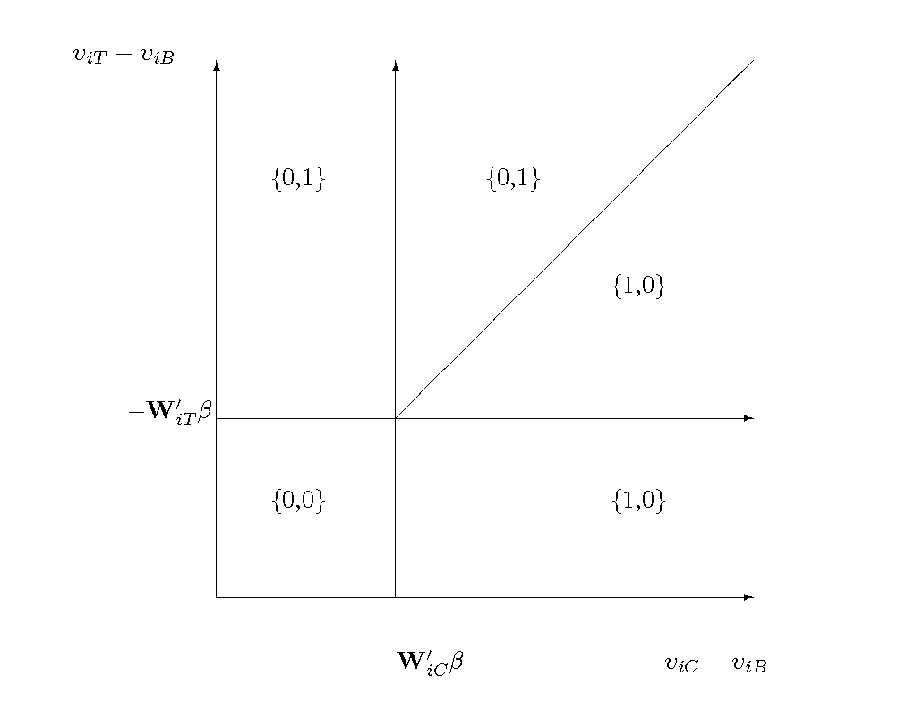
The Figure 4 depicts the three choices as a function of the unobserved characteristics. If the relative unobserved characteristics of both choices are low enough, then neither is chosen. That is, the individual chooses Bus. The individual chooses Car if the relative unobserved characteristic is higher for Car than it is for Train.

Multinomial Probit

When there are three choices, the multinomial normal is a bivariate normal. The bivariate probit model assumes \(\{\upsilon_{iC} - \upsilon_{iB}, \upsilon_{iT} - \upsilon_{iB}\} \sim \mathcal{N}(\mathbf{\mu}, \mathbf{\Sigma})\), where \(\mathbf{\mu} = \{0, 0\}\) and

\[ \mathbf{\Sigma} = \left [\begin{array}{ll} 1 & \rho\\ \rho & 1 \end{array} \right ] \tag{30}\]

and \(\rho \in [-1, 1]\) is the correlation between the unobserved characteristics determining the relative demand for cars and trains. Note that the variance of the relative unobserved characteristics is not identified by the choice data and is assumed to be 1.

The simplest case is the probability of observing Bus (\(\{0,0\}\)).

\[ \Pr(y_i = \{0,0\} | \mathbf{W}, \beta, \rho) = \int_{-\infty}^{-\mathbf{W}_{iC}'\beta} \Phi \left(\frac{-\mathbf{W}_{iT}'\beta - \rho \upsilon_1}{\sqrt(1 - \rho^2)} \right) \phi(\upsilon_1) d \upsilon_1 \tag{31}\]

Simplest, not simple. A word to the wise, writing out multivariate probits is a good way to go insane.

There is a lot to unpack in Equation 31. First, it is written out in a way that is going to allow “easy” transition to R code. The probability in question is a joint probability over the two relative unobserved characteristics. This joint probability can be written as a mixture distribution of the probability of not choosing Train conditional on the unobserved characteristic for the choice of Car. Next, the probability over not choosing Train is written out using a standard normal distribution. This is useful for programming it up in R. Lastly, because the unobserved characteristics may be correlated, the variable needs to be normalized, where the distribution of the conditional unobserved characteristic has a mean of \(\rho \upsilon_1\) and a variance of \(1 - \rho^2\).¹⁸

The probability of observing the choice of Car (\(\{1,0\}\)) is similar, although even more complicated. Consider Figure 4. We are interested in measuring the trapezoid that is below the diagonal line and to the right of the vertical line.

\[ \Pr(y_i = \{1,0\} | \mathbf{W}, \beta, \rho) = \int_{-\mathbf{W}_{iC}'\beta}^{\infty} \Phi \left(\frac{-\mathbf{W}_{iT}'\beta + (1 - \rho) \upsilon_1}{\sqrt(1 - \rho^2)} \right) \phi(\upsilon_1) d \upsilon_1 \tag{32}\]

Now the choice of Car is determined by both the relative value of Car to Bus and the relative value of Car to Train. If the unobserved characteristic associated with the Car choice is high, then the unobserved characteristic associated with Train does not have to be that low for Car to be chosen.

Multinomial Probit in R

The Equation 31 and Equation 32 have been written in a way to suggest pseudo-code for the bivariate probit. Note how the integral is done. The program takes a set of draws from a standard normal distribution and then for each draw it calculates the appropriate probabilities. After the loop has finished, the probabilities are averaged. This approach gives relatively accurate estimates even with relatively small numbers of loops. Even so, the computational burden of this estimator is large. Moreover, this burden increases dramatically with each choice that is added to the problem.

f_biprobit <- function(para, Y, W1, W2, K = 10) {
  # K is a counter for the number of draws from the normal
  # distribution - more draws gives greater accuracy 
  # but slower computational times.
  # function setup
  set.seed(123456789)  # helps the optimizer work better.
  eps <- 1e-20  # used below to make sure the logs work.
  W1 <- cbind(1,W1)
  W2 <- cbind(1,W2)
  N <- dim(Y)[1]
  J <- dim(W1)[2]
  rho <- exp(para[1])/(1 + exp(para[1]))
  # the "sigmoid" function that keeps value between 0 and 1.
  # It assumes that the correlation is positive.
  beta <- para[2:(J+1)]
  # integration to find the probabilities
  u <- rnorm(K)
  p_00 <- p_10 <- rep(0, N)
  for (uk in u) {
    uk0 <- uk < -W1%*%beta
    p_00 <- p_00 + 
      uk0*pnorm((-W2%*%beta - rho*uk)/((1 - rho^2)^(.5)))
    p_10 <- p_10 + (1 - uk0)*pnorm(((W1 - W2)%*%beta + 
                            (1 - rho)*uk)/((1 - rho^2)^(.5)))
  }
  # determine the likelihood
  log_lik <- (Y[,1]==0 & Y[,2]==0)*log(p_00/K + eps) +
    (Y[,1]==1 & Y[,2]==0)*log(p_10/K + eps) +
    (Y[,1]==0 & Y[,2]==1)*log(1 - p_00/K - p_10/K + eps)
  return(-sum(log_lik))
}

Multinomial Logit

Given the computational burden of the multivariate normal, particularly as the number of choices increase, it is more common to assume a multinomial logit. This model assumes that the unobserved characteristic affecting the choice between Car and Bus is independent of the unobserved characteristic affecting the choice between Car and Train.¹⁹

\[ \Pr(y_i = \{1,0\} | \mathbf{W}, \beta) = \frac{\exp(\mathbf{W}_{iC}' \beta)}{1 + \sum_{j \in \{C,T\}}\exp(\mathbf{W}_{ij} ' \beta)} \tag{33}\]

As above, a maximum log-likelihood algorithm is used to estimate the multinomial logit.

Multinomial Logit in R

Starting with the bivariate probit and Equation 33, we can write out the multinomial logit with three choices.

f_logit <- function(beta,Y,W1,W2) {
  eps <- 1e-20 # so we don't take log of zero.
  Y1 <- as.matrix(Y) 
  W1 <- as.matrix(cbind(1,W1))
  W2 <- as.matrix(cbind(1,W2))
  p_10 <- 
    exp(W1%*%beta)/(1 + exp(W1%*%beta) + exp(W2%*%beta))
  p_01 <- 
    exp(W2%*%beta)/(1 + exp(W1%*%beta) + exp(W2%*%beta))
  p_00 <- 1 - p_10 - p_01
  log_lik <- (Y[,1]==0 & Y[,2]==0)*log(p_00 + eps) +
    (Y[,1]==1 & Y[,2]==0)*log(p_10 + eps) +
    (Y[,1]==0 & Y[,2]==1)*log(p_01 + eps)
  return(-sum(log_lik))
}

Notice that, unlike the multinomial probit, we do not need to take random number draws. Calculating the probabilities is much simpler and computationally less intensive.

Simulating Multinomial Choice

Now we can compare the two methods. The simulation uses a bivariate normal distribution to simulate individuals choosing between three options. The simulation also assumes that the unobserved characteristics are correlated between choices.

require(mvtnorm)  

Loading required package: mvtnorm

Warning: package 'mvtnorm' was built under R version 4.4.1

# this package creates multivariate normal distributions
set.seed(123456789)
N <- 1000
mu <- c(0,0)
rho <- 0.1 # correlation parameter
Sig <- cbind(c(1,rho),c(rho,1))
u <- rmvnorm(N, mean = mu, sigma = Sig)
# relative unobserved characteristics of two choices
x1 <- matrix(runif(N*2), nrow=N)
x2 <- matrix(runif(N*2), nrow=N)
# relative observed characteristics of two choices.
a <- -1
b <- -3
c <- 4
U <- a + b*x1 + c*x2 + u
Y <- matrix(0, N, 2)
Y[,1] <- U[,1] > 0 & U[,1] > U[,2]
Y[,2] <- U[,2] > 0 & U[,2] > U[,1]
par1 <- c(log(rho),a,b,c)
a1 <- optim(par=par1, fn=f_biprobit,Y=Y,
            W1=cbind(x1[,1],x2[,1]),
            W2=cbind(x1[,2],x2[,2]),K=100,
            control = list(trace=0,maxit=1000))
par2 <- c(a,b,c)
b1 <- optim(par=par2, fn=f_logit,Y=Y,W1=cbind(x1[,1],x2[,1]),
            W2=cbind(x1[,2],x2[,2]),
            control = list(trace=0,maxit=1000))
a1$par[2:4]

[1] -1.039715 -2.819453  3.887579

b1$par[1:3]

[1] -1.591007 -4.976470  6.687181

At 100 draws, the bivariate probit estimator does pretty well, with \(\hat{\beta} = \{-1.04, -2.82, 3.89\}\) compared to \(\beta = \{-1, -3, 4\}\). The logit model doesn’t do nearly as well. This isn’t surprising given that the assumptions of the model do not hold in the simulated data. Even still it gets the signs of the parameters and you can see that it solves much quicker than the bivariate probit.

Demand for Rail

In McFadden’s analysis, policy makers were interested in how many people would use the new BART rail system. Would there be enough users to make such a large infrastructure project worthwhile? This question remains relevant for cities across the US. Many large US cities like New York, Chicago and Boston, have major rail infrastructure, while many smaller US cities do not. For these smaller cities, the question is whether building a substantial rail system will lead to an increase in public transportation use.

To analyze this question we can use data from the National Household Travel Survey.²⁰ In particular, the publicly available household component of that survey. The data provides information on what mode of transport the household uses most days; car, bus or train. It contains demographic information such as home ownership, income, and geographic information such as rural and urban residence. Most importantly for our question, the data provides a measure of how dense the rail network is in the location.

The section uses logit and probit models to estimate the demand for cars in “rail” cities and “non-rail” cities. It estimates the multinomial version of these models for “rail” cities. It then takes those parameter estimates to predict demand for rail in “non-rail” cities.

National Household Travel Survey

The following code brings in the data and creates variables. It creates the “choice” variables for transportation use. Note that households may report using more than one mode, but the variables are defined exclusively. The code also adjusts variables for missing. The data uses a missing code of -9. This would be used as a value if it is not replaced with NA.

x <- read.csv("hhpub.csv", as.is = TRUE)
x$choice <- NA
x$choice <- ifelse(x$CAR==1,"car",x$choice)
x$choice <- ifelse(x$BUS==1,"bus",x$choice)
x$choice <- ifelse(x$TRAIN==1,"train",x$choice)
# Note that this overrules the previous choice.
x$car1 <- x$choice=="car"
x$train1 <- x$choice=="train"
# adjusting variables to account for missing.
x$home <- ifelse(x$HOMEOWN==1,1,NA)
x$home <- ifelse(x$HOMEOWN>1,0,x$home)
# home ownership
x$income <- ifelse(x$HHFAMINC > 0, x$HHFAMINC, NA)
# household income
x$density <- ifelse(x$HTPPOPDN==-9,NA,x$HTPPOPDN)/1000
# missing is -9.
# population density
# dividing by 1000 makes the reported results look nicer.
x$urban1 <- x$URBAN==1  # urban versus rural
y <- x[x$WRKCOUNT>0 & (x$MSACAT == 1 | x$MSACAT == 2),]
# limit to households that may commute and those that 
# live in some type of city.
y$rail <- y$RAIL == 1
# an MSA with rail
index_na <- is.na(rowSums(cbind(y$car1,y$train1,
                                y$home,y$HHSIZE,y$income,
                                y$urban1,y$density,y$MSACAT,
                                y$rail)))==0
y <- y[index_na,] # drop missing

How different are “rail” cities from “non-rail” cities? The plan is to use demand estimates for cars, buses, and rail in cities with rail networks to predict demand for rail in other cities. However, cities with and without rail may differ in a variety of ways which may lead to different demand for rail between the two types of cities.

vars <- c("car1","train1","home","HHSIZE","income",
          "urban1","density")
summ_tab <- matrix(NA,length(vars),2)
for (i in 1:length(vars)) {
  summ_tab[i,1] <- mean(y[y$rail==1,colnames(y)==vars[i]])
  summ_tab[i,2] <- mean(y[y$rail==0,colnames(y)==vars[i]])
}
row.names(summ_tab) <- vars
colnames(summ_tab) <- c("Rail","No Rail")

Table 2: Means by rail network density.

	Rail	No Rail
car1	0.8779250	0.9738615
train1	0.0966105	0.0100361
home	0.7301273	0.7492306
HHSIZE	2.4878699	2.4624203
income	7.5188403	7.0545519
urban1	0.9102719	0.8697533
density	7.5590760	4.6619363

The Table 2 presents summary results for each type of city. It shows that in cities with rail networks about 10% of the population uses trains most days, while it is only 1% of those in cities without dense rail networks. The different cities also differ in other ways including income and population density.

What would happen to the demand for rail if a city without one built it? Would demand increase to 10% as it is in cities with rail networks? Or would demand be different due to other differences between the cities?

Demand for Cars

We can also look at how the demand for cars varies between the two types of cities.

# Without Rail
y_nr <- y[y$rail == 0,]
glm_nr <- glm(car1 ~ home + HHSIZE + income + urban1 +
                density, data = y_nr, 
              family=binomial(link=logit))

# With Rail
y_r <- y[y$rail == 1,]
glm_r <- glm(car1 ~ home + HHSIZE + income + urban1 + 
               density, data = y_r, 
             family=binomial(link=logit))

Table 3: Logit estimates of demand for cars. Model (1) is demand in cities without a dense rail network. Model (2) is demand in cities with a rail network.

	(1)	(2)
(Intercept)	3.775	3.506
	(0.270)	(0.211)
home	0.633	0.498
	(0.095)	(0.071)
HHSIZE	-0.018	0.050
	(0.033)	(0.026)
income	0.133	-0.068
	(0.019)	(0.013)
urban1TRUE	-1.160	-0.312
	(0.245)	(0.187)
density	-0.055	-0.109
	(0.008)	(0.003)
Num.Obs.	22419	11624
AIC	5129.3	7005.1
BIC	5177.5	7049.2
Log.Lik.	-2558.673	-3496.533
RMSE	0.16	0.29

While Table 3 shows that demand for cars varies given different access to rail. It is not clear how to interpret the coefficient estimates. There are lots of differences between the two types of cities, including the choices available to commuters. Nevertheless, we see the demand increasing in home ownership and decreasing in density.

Estimating Demand for Rail

We can set up the McFadden demand model for cars, buses and trains. The utility of car and train is relative to bus. Note that the value of train is assumed to be a function of density. The assumption is that trains have fixed station locations and in more dense cities, these locations are likely to be more easily accessible to the average person.

X_r_car <- cbind(y_r$home, y_r$HHSIZE, y_r$income, 
                 y_r$urban1,0)
X_r_train <- cbind(0,0,0,0,y_r$density)
# train value is assumed to be determined by 
# population density.
Y1_r <- cbind(y_r$choice=="car",y_r$choice=="train")

The following presents the optimization procedure for the two multinomial choice models. Each uses the initial probit or logit model for starting values on the \(\beta\) term. To be clear, the estimation is done on cities with rail networks.

par1 <- c(0,glm_r$coefficients)
a1 <- optim(par=par1,fn=f_biprobit,Y=Y1_r,W1=X_r_car,
            W2=X_r_train,K=100,control=list(trace=0,
                                            maxit=10000))
par2 <- glm_r$coefficients
a2 <- optim(par=par2,fn=f_logit,Y=Y1_r,W1=X_r_car,
            W2=X_r_train,control=list(trace=0,maxit=10000))

Predicting Demand for Rail

Once we estimate demand for car, bus, and rail in cities with rail networks, we can use the estimated parameters to predict demand for rail in a non-rail city. To do this, we combine the parameter estimates from rail cities with the observed characteristics of households in non-rail cities. This is done for both the multinomial probit and the multinomial logit.

X_nr_car <- cbind(1,y_nr$home, y_nr$HHSIZE, y_nr$income,
                  y_nr$urban1,0)
X_nr_train <- cbind(1,0,0,0,0,y_nr$density)
# Probit estimate
set.seed(123456789)
rho <- exp(a1$par[1])/(1 + exp(a1$par[1]))
beta <- a1$par[2:length(a1$par)]
W1 <- X_nr_car
W2 <- X_nr_train
K1 = 100
u1 <- rnorm(K1)
p_00 <- p_10 <- rep(0, dim(W1)[1])
for (uk in u1) {
  uk0 <- uk < -W1%*%beta
  p_00 <- p_00 + 
    uk0*pnorm((-W2%*%beta - rho*uk)/((1 - rho^2)^(.5)))
  p_10 <- p_10 + 
    (1 - uk0)*pnorm(((W1 - W2)%*%beta +
                       (1 - rho)*uk)/((1 - rho^2)^(.5)))
}
p_train_pr <- (K1 - p_00 - p_10)/K1
mean(p_train_pr)

[1] 0.08872575

# Logit estimate
p_train_lg_top <- exp(X_nr_train%*%a2$par)
p_train_lg_bottom <- 1 + exp(X_nr_car%*%a2$par) + 
  exp(X_nr_train%*%a2$par)
p_train_lg <- p_train_lg_top/p_train_lg_bottom
mean(p_train_lg)

[1] 0.08313867

If a city without rail built one, the demand for rail would increase substantially. It would increase from 1% to either 8.3% or 8.9%, depending upon the estimator used. A substantial increase, almost to the 10% we see for cities with rail. Do you think this evidence is enough to warrant investment in rail infrastructure by smaller US cities?

Discussion and Further Reading

The first part of the book presented methods that focused on the use of experimentation, or lack thereof. This part focuses on methods based on economic theory. This chapter discusses how the economic assumption of revealed preference can be used to identify the policy parameters of interest. The Nobel Prize winning economist, Daniel McFadden, showed how combining economic theory and survey data could provide better predictions of demand for new products.

This chapter presented the standard discrete choice models of the logit and probit. The chapter introduces the maximum likelihood algorithm. It shows how this algorithm can be used to estimate OLS, logit and probit models.

The application of the logit and probit is to demand estimation. While these are standard methods, the reader should note that they are not really the way modern demand analysis is done. The chapter assumes that prices (or product characteristics) are exogenous. Modern methods use an IV approach to account for the endogeneity of prices. In particular, the ideas of Berry, Levinsohn, and Pakes (1995) have become standard in my field of Industrial Organization. Chapter 7 discusses this approach in more detail.

References

Berry, Steven, James Levinsohn, and Ariel Pakes. 1995. “Automobile Prices in Market Equilibrium.” Econometrica 60 (4): 889–917.

Goldberger, Arthur. 1991. A Course in Econometrics. Harvard University Press.

Manski, Charles F. 1990. “Nonparametric Bounds on Treatment Effects.” American Economic Review Papers and Proceedings 80: 319–23.

McFadden, Daniel. 1974. “The Measurement of Urban Travel Demand.” Journal of Public Economics 3: 303–28.

Nevo, Aviv. 2000. “A Practioner’s Guide to Estimation of Random-Coefficients Logit Models of Demand.” Journal of Economics and Management Strategy 9 (4): 513–48.

Footnotes

1. https://www.nobelprize.org/prizes/economic-sciences/2000/mcfadden/lecture/

2. https://www.ftc.gov/system/files/documents/public_statements/295971/130103googlesearchstmtofcomm.pdf

3. This is a standard assumption in economics. It means that the unobserved utility can be thought of as money.

4. In machine learning, discrete choice is referred to as a classification problem.

5. This is actually a probit model presented in more detail below.

6. Independent means that if I know the first two coin tosses result in Heads, the probability of a Head in the third coin toss is the same as if I saw two Tails or any other combination. The previous coin toss provides no additional information about the results of the next coin toss, if the true probability is known.

7. See discussion of the analogy principle in Appendix A.

8. Optimums do not vary with monotonic transformations.

9. The function optimize() is used when optimizing over one variable, while optim() is used for optimizing over multiple variables.

10. This has to do with the ability of this function to quickly run through vectors. See Appendix B for a discussion of programming in R.

11. This assumes that the outcomes are independent and identically distributed.

12. See the formula for standard normal.

13. Thanks to Joris Pinkse for pointing this issue out.

14. This issue is discussed in Chapter 1.

15. Note in the simulated data, the \(\upsilon_{iA}\) term is dropped so that the assumption holds.\index{subjectindex}{standard normal distribution

16. It is used in neural network estimation models. In machine learning this is called a “sigmoid” function.

17. It is this property that makes it useful as an “activation” function in neural network models.

18. See Goldberger (1991) for the best exposition that I am aware of.

19. The logit function has the advantage that it is very easy to estimate, but the disadvantage that places a lot of restrictions on how preferences determine choices. Given these restrictions there is interest in using more flexible models such as the multi-layered logit (deep neural-network) or the mixed logit model discussed in Nevo (2000).

20. https://nhts.ornl.gov/