Instrumental Variables

Author

Christopher P. Adams

Introduction

Despite being a relatively recent invention, the instrumental variable (IV) method has become a standard technique in microeconometrics.¹ The IV method provides a potential solution for one of the two substantive restrictions imposed by OLS. OLS requires that the unobserved characteristic of the individual enters into the model independently and additively. The IV method allows the estimation of causal effects when the independence assumption does not hold.

Consider again a policy in which Vermont makes public colleges free. Backers of such a policy believe that it will encourage more people to attend college. Backers also note that people who attend college earn more money. But do the newly encouraged college attendees earn more money?

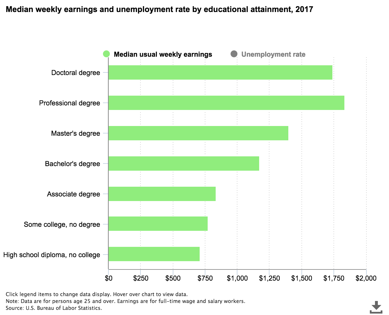
Figure 1: Chart of median weekly earnings by education level 2017 from Bureau of Labor Statistics.

Figure 1 presents median weekly earnings by education level for 2017. It shows that those with at least a Bachelor’s Degree earn substantially more than those who never attended college. Over $1,100 per week compared to around $700. However, this is not the question of interest.
The policy question is whether encouraging more people to attend college will lead these people to earn more. The problem is that people who attend college are different from people who do not attend college. Moreover, those differences lead to different earnings.

In the previous chapter we solve this omitted variable problem by estimating $c$ and $e$. Here, we cannot use this method because we do not observe $U$. This chapter aims to solve the backdoor problem by using instrumental variables.

The chapter presents a general model of the IV estimator. It then presents a version of the estimator for R. The estimator is used to analyze returns to schooling and replicates Card (1995). The chapter uses the data to test whether the proposed instrumental variables satisfy the assumptions. The chapter ends with a discussion of an alternative IV estimator called the local average treatment effect (LATE) estimator. This estimator relaxes the additivity assumption.

A Confounded Model

The problem with comparing earnings from college attendees with those that have not attended college is confounding. There may be some unobserved characteristic associated with both attending college and earning income.

DAG of Confounded Model

flowchart TD
  X(X) -- b --> Y(Y)
  U(U) -- c --> Y
  U -- e --> X

Figure 2: Confounded graph.

Consider the graph presented in Figure 2. We want to estimate the causal relationship between $X$ and $Y$. $X$ may represent college attendance and $Y$ represents weekly earnings. The arrow from $X$ to $Y$ represents the causal effect of $X$ on $Y$. This effect is denoted by $b$. Here, $b$, represents the increase in earnings due to a policy that increases the propensity to attend college. In order to evaluate the policy, we need to estimate $b$.

In Chapters 1 and 2 we saw a similar figure. This time we have an arrow from $U$ to $X$. This extra arrow means the unobserved characteristics can determine the value of the policy variable. People who attend college may earn more than people who do not attend college for reasons that have nothing at all to do with attending college.

If our data is represented by Figure 2 we can try to estimate $b$ by regressing $Y$ on $X$. Doing so, however, will not give an estimate of $b$. Rather it will give an estimate of $b + \frac{e}{c}$. This is due to the backdoor problem. The issue is that there are two pathways connecting $X$ to $Y$. One is the “front door” as represented by the arrow directly from $X$ to $Y$ with a weight of $b$. The second is the backdoor, which follows the backward arrow from $X$ to $U$ with the weight of $\frac{1}{c}$ and then the forward arrow from $U$ to $Y$, with the weight of $e$.

A Linear Confounded Model

We can write our confounded model with algebra.

\[ y_i = a + b x_i + e \upsilon_{1i}\\ \\ x_i = f + d z_i + \upsilon_{2i} + c \upsilon_{1i} \tag{1}\]

where $y_i$ represents individual $i$’s income, $x_i$ is their education level, and $\upsilon_{1i}$ and $\upsilon_{2i}$ are unobserved characteristics that determine income and education level respectively. We are interested in estimating $b$. This is the same as the model we saw in the previous chapters. The difference here is that there is an additional equation.

To see the problem with OLS, rearrange the second equation and substitute it into the first equation.

\[ y_i = a + b x_i + e \left(\frac{x_i - f - d z_i - \upsilon_{2i}}{c}\right) \tag{2}\]

If we run OLS, we estimate the coefficient on $x$ as $b + \frac{e}{c}$, not $b$. In Chapter 2 we looked to solve this problem by estimating $e$ and $c$. We can’t do that here because we do not observe $\upsilon_{1i}$. The solution proposed in this chapter is called instrumental variables.

Simulation of Confounded Data

set.seed(123456789)  
N <- 1000
a <- 2
b <- 3
c <- 2
e <- 3
f <- -1
d <- 4
z <- runif(N)
u_1 <- rnorm(N, mean=0, sd=3)
u_2 <- rnorm(N, mean=0, sd=1) 
x <- f + d*z + u_2 + c*u_1 
y <- a + b*x + e*u_1
lm1 <- lm(y ~ x)

The simulated data is generated from the model presented above. The causal effect of $x$ on $y$ is $b = 3$. We see that $u_1$ affects both $x$ and $y$. A standard method for estimating the causal effect of $X$ on $Y$ is to use OLS. (tab-lm1_2?) presents the OLS estimate of the simulated data. The table shows that the estimated relationship is 4.38. It is much larger in magnitude than the true value of $3$. It is closer to the backdoor relationship of $b + \frac{e}{c} = 4.5$.

Loading required package: knitr

OLS estimate with confounded data.

	Estimate	Std. Error	t value	Pr(>\|t\|)
(Intercept)	0.5113529	0.0706473	7.238109	0
x	4.4090257	0.0111962	393.797828	0

We can estimate $b$, but our estimate is wrong.

IV Estimator

Perhaps the most common solution to confounding used in microeconometrics is the IV estimator. This section formally presents the estimator and illustrates it with the simulated data.

Graph Algebra of IV Estimator

Figure 3 represents the confounded data. It shows that the instrumental variable ($Z$) has a direct causal effect on $X$ but is not determined by the unobserved characteristic. There is an arrow from $Z$ to $X$ and an arrow from $U$ to $X$, but no arrow from $U$ to $Z$.

flowchart TD
  Z(Z) -- d --> X(X)
  X -- b --> Y(Y)
  U(U) --> Y
  U --> X

Figure 3: Experimental graph.

“Graph algebra” provides a solution. If we are interested in estimating $b$, we can do so by estimating the relationship between $Z$ and $Y$. That effect is given by $b \times d$. We can estimate $d$ by running a regression of $X$ on $Z$. Thus dividing the result of the first regression by the result of the second regression gives the answer. If the unobserved characteristic affects the explanatory variable additively then the division procedure can be used to estimate the true causal relationship.

In the medical literature the first regression is called the intent to treat regression. The name comes from randomized controlled trials where patients are randomly assigned to alternative treatments, say a new cancer therapy versus the standard of care. Unfortunately, patients may not accept their treatment assignment. They may leave the trial or they may switch to the non-assigned treatment. In that case $Z$ represents the randomization method while $X$ represents the *actual} treatment received. By regressing $Z$ on $Y$ we are estimating causal effect of the initial randomized assignment. We are estimating the “intent” of the trial. Often only this estimate ($d \times b$) is presented, rather than effect of interest ($b$). See for example the analysis of commitment savings devices in the next chapter (Ashraf, Karlan, and Yin 2006).

Properties of IV Estimator

In the standard analysis, an instrumental variable has three properties.

The variable directly affects the policy variable of interest ($Z \rightarrow X$).
The variable is independent of the unobserved characteristics that affect the policy variable and the outcome of interest ($U \not \rightarrow Z$).²
The variable affects the policy variable independently of the unobserved effect ($X = d Z + U$).

If we have a variable that satisfies these three properties, then we can use the graph algebra to estimate the causal effect of interest. Below we discuss how restrictive these assumptions are and test whether they hold in the data.

IV Estimator with Standard Algebra

A simple IV estimator is derived by rearranging the equations above ( (Equation 1)). We can determine the relationship between $z_i$ and $y_i$ by substituting $x_i$ into the first equation.

\[ y_i = a + b (f + d z_i + u_{2i} + c u_{1i}) + e u_{1i}\\ \\ \mbox{, or }\\ y_i = a + b f + b d z_i + b u_{2i} + b c u_{1i} + e u_{1i} \tag{3}\]

We can use OLS to give an unbiased estimate of the relationship between $z_i$ and $y_i$, which is $b d$ in the true model. The problem is that we are not interested in $b d$, we are interested in knowing $b$. (Equation 1) shows we can use OLS to estimate the relationship between $z_i$ and $x_i$. This gives an estimate of $d$. Thus, the division of the first estimate by the second gives an estimate of $b$.

Simulation of an IV Estimator

To illustrate the estimator, note that in the simulated data there exists a third variable $z$. This variable determines $x$ but does not directly determine $y$ and is independent of the unobserved characteristic ($\upsilon$).

Consider what happens if we run an OLS regression of $y$ on $z$ and a separate OLS regression of $x$ on $z$.

bd_hat <- lm(y ~ z)$coef[2]
d_hat <- lm(x ~ z)$coef[2]
# picking the slope coefficient from each regression
bd_hat/d_hat

       z 
3.015432

If we take the coefficient estimate from the first regression and divide that number by the coefficient estimate from the second regression, we get an estimate that is close to the true relationship. This is not coincidental. The observed characteristic, $z$, has the properties of an instrumental variable.

The procedure works well, but only if we want to instrument for one variable.

IV Estimator with Matrix Algebra

If we want to instrument for more than one variable we need matrix algebra. In matrix algebra, the model above is as follows.

\[ \mathbf{y} = \mathbf{X} \mathbf{\beta} + \mathbf{u} \tag{4}\]

where $\mathbf{y}$ is a $100 \times 1$ vector of the outcome of interest $y_i$, $\mathbf{X}$ is a $100 \times 2$ matrix of the observed explanatory variables $\{1, x_i\}$, $\mathbf{\beta}$ is a $2 \times 1$ vector of the model parameters $\{a, b\}$ and $\mathbf{u}$ is a $100 \times 1$ vector of the error term $u_i$.

In addition, there is a relationship between the instrumental variables and the explanatory variables.

\[ \mathbf{X} = \mathbf{Z} \Delta + \mathbf{E} \tag{5}\]

where $\mathbf{Z}$ is a $100 \times 2$ matrix of the instrumental variables $\{1, z_i\}$, $\Delta$ is a $2 \times 2$ matrix of the relationship between the explanatory variables and the instrumental variables, and $\mathbf{E}$ is a $100 \times 2$ matrix of unobserved characteristics determining the explanatory variables.

We can rearrange (Equation 5) to determine $\Delta$ as a function of the observed and unobserved variables.

\[ \Delta = (\mathbf{Z}' \mathbf{Z})^{-1} \mathbf{Z}' \mathbf{X} - (\mathbf{Z}' \mathbf{Z})^{-1} \mathbf{Z}'\mathbf{E} \tag{6}\]

Note that we use the exact same matrix procedure as we use for OLS in Chapter 1. There we “divided by” $\mathbf{X}$, here we “divide by” $\mathbf{Z}$.³ The matrix $\mathbf{Z}'$ is the matrix transpose. By pre-multiplying we have a square matrix that may be invertible. It is assumed that the matrix $\mathbf{Z}$ is full-column rank.

A few more steps and we have our estimator. If we substitute (Equation 5) into (Equation 4) we have our intent to treat regression.

\[ \mathbf{y} = \mathbf{Z} \Delta \beta + \mathbf{E} \beta + \mathbf{u} \tag{7}\]

Rearranging this equation we can get an estimator for the coefficients ($\Delta \beta$).

\[ \Delta\beta = (\mathbf{Z}' \mathbf{Z})^{-1} \mathbf{Z}'\mathbf{y} - (\mathbf{Z}' \mathbf{Z})^{-1} \mathbf{Z}'\mathbf{V} \beta - (\mathbf{Z}' \mathbf{Z})^{-1} \mathbf{Z}'\mathbf{u} \tag{8}\]

Substituting (Equation 6) into this equation and simplifying, we have the following relationship.

\[ \beta = (\mathbf{Z}' \mathbf{X})^{-1} \mathbf{Z}'\mathbf{y} - (\mathbf{Z}' \mathbf{X})^{-1} \mathbf{Z}'\mathbf{u} \tag{9}\]

From (Equation 9) we have our instrumental variable estimator.

\[ \hat{\beta}_{IV} = (\mathbf{Z}' \mathbf{X})^{-1} \mathbf{Z}'\mathbf{y} \tag{10}\]

Remember, we don’t observe the last part of (Equation 9). This means that our estimate of $\hat{\beta}_{IV}$ will not be equal to $\beta$. The question is when they are likely to be close to each other.⁴

This generalizes OLS. If the instrumental variable matrix ($\mathbf{Z}$) is equal to the explanatory variable matrix ($\mathbf{X}$) then this is just our OLS estimator. This relationship makes it clear that OLS assumes that each explanatory variable is independent of the unobserved characteristic. There is no arrow from $U$ to $X$. More generally, the matrix of instrumental variables must be the same size as the matrix of explanatory variables. Each explanatory variable must either have an assigned instrument or must be an instrument for itself.⁵

Two-Stage Least Squares

A common algorithm for IV is two-stage least squares. This algorithm operationalizes the matrix algebra steps above. From (Equation 6) we have a first-stage estimator.

\[ \hat{\Delta} = (\mathbf{Z}' \mathbf{Z})^{-1} \mathbf{Z}' \mathbf{X} \tag{11}\]

That is, we regress the set of instruments (exogenous variables) on the set of endogenous variables. Note that the result is a matrix, rather than a vector in the standard OLS model.

We can use this estimate in the second-stage regression. We can go to (Equation 7) and replace the $\mathbf{Z} \Delta$ with $\mathbf{Z} \hat{\Delta}$. That is, we replace the endogenous variables with their predicted values.

I have not coded up the two-stage least squares algorithm. We use the algorithm derived from the matrix algebra. Can you code the two-stage least squares estimator? How does it compare to the estimator below?

IV Estimator in `R`

We can use (Equation 10) as pseudo-code for the instrumental variable estimator. Note that while the OLS estimator gives estimates that diverge substantially from the true values for both the intercept and the slope, the IV estimates are a lot closer to the true values.

X <- cbind(1,x) # remember the column of 1's for the intercept
Z <- cbind(1,z) # remember Z same size as X
beta_hat_ols <- solve(t(X)%*%X)%*%t(X)%*%y
beta_hat_iv <- solve(t(Z)%*%X)%*%t(Z)%*%y
beta_hat_ols

       [,1]
  0.5113529
x 4.4090257

beta_hat_iv

      [,1]
  1.715181
x 3.015432

Bootstrap IV Estimator for `R`

The following bootstrap IV estimator defaults to an OLS estimator. It uses the matrix algebra above to create a function that we can use on various problems. In R the function() operator is used to create an object that takes inputs and produces an output. In this case, it takes in our data and produces an instrumental variable estimate.

To use this estimator, you can copy the code and then “run” that proportion of the code defining the function. Once that is done, you can call the function in your R script.

lm_iv <- function(y, X_in, Z_in = X_in, Reps = 100, 
                  min_in = 0.05, max_in = 0.95) {
  # takes in the y variable, x explanatory variables
  # and the z variables if available.
  # The "=" creates a default value for the local variables.
  
  # Set up 
  set.seed(123456789)
  X <- cbind(1,X_in)  # adds a column of 1's the matrix
  Z <- cbind(1,Z_in) 
  

  # Bootstrap
  bs_mat <- matrix(NA,Reps,dim(X)[2]) 
  # dim gives the number of rows and columns of a matrix.
  # the second element is the number of columns.
  N <- length(y) # number of observations
  for (r in 1:Reps) {
    index_bs <- round(runif(N, min = 1, max = N))
    y_bs <- y[index_bs]  # note Y is a vector
    X_bs <- X[index_bs,]
    Z_bs <- Z[index_bs,]
    bs_mat[r,] <- solve(t(Z_bs)%*%X_bs)%*%t(Z_bs)%*%y_bs
  }
  
  # Present results
  tab_res <- matrix(NA,dim(X)[2],4)
  tab_res[,1] <- colMeans(bs_mat)
  for (j in 1:dim(X)[2]) {
    tab_res[j,2] <- sd(bs_mat[,j])
    tab_res[j,3] <- quantile(bs_mat[,j],min_in)
    tab_res[j,4] <- quantile(bs_mat[,j],max_in)
  }
  colnames(tab_res) <- c("coef","sd", as.character(min_in),
                          as.character(max_in))
  return(tab_res)
  # returns the tab_res matrix.
}

The function takes as inputs the vector of outcome variables ($y$), a matrix of explanatory variables (the $X$s), and a matrix of instruments ($Z$s).⁶ It defaults to allowing $\mathbf{X} = \mathbf{Z}$. It also assumes that the matrix of instruments is the exact same dimension as the matrix of explanatory variables. The function then tidies up by adding the column of 1s to both the matrix of explanatory variables and the matrix of instruments. The function accounts for sampling error by using the bootstrap methodology.⁷ The bootstrap creates pseudo-random samples by re-sampling the original data and re-estimating the model on each new pseudo-sample. In each case, it uses the matrix algebra presented above to calculate the estimator.

print(lm_iv(y,x), digits = 3)  # OLS

      coef     sd  0.05  0.95
[1,] 0.513 0.0729 0.396 0.643
[2,] 4.409 0.0109 4.394 4.427

print(lm_iv(y,x,z), digits = 3) # IV

     coef    sd 0.05 0.95
[1,] 1.83 0.377 1.30 2.43
[2,] 2.96 0.286 2.45 3.37

We can compare the IV and OLS estimators on the simulated data. Using the IV estimator with the simulated data shows that the OLS estimates are biased and that the true values do not lie within the 90% confidence interval. The IV estimates do better.

Returns to Schooling

Chapters 1 and 2 discussed how Canadian labor economist, Berkeley’s David Card, used OLS to estimate returns to schooling. Card finds that an extra year of schooling increases income by approximately 7.5%. Card points out that this estimate may be biased and argues for using the instrumental variable approach.

flowchart TD
  Z(Distance to College) -- delta --> X(Education)
  X -- beta --> Y(Income)
  U(Unobserved Characteristics) --> Y
  U --> X

Figure 4: Returns to schooling graph.

The unobserved characteristics of the young men may determine both the amount of education that they get and the income they earn. In Figure 4, the problem is illustrated with a causal arrow running from the unobserved characteristic to both income and education. For example, young men from wealthier families may be more likely to go to college because their families can afford it. In addition, these young men may go into well paying jobs due to family connections. In this case, the observed positive relationship we see between education and income may be due to the wealth of the young man’s family rather than the education itself. The effect of the confounding is that we get an inaccurate estimate of $\beta$. If a policy is designed to increase education it won’t have the expected effect on income. OLS may not give an accurate estimate of $\beta$.

Distance to College as an Instrument

Card (1995) argues that young men who grow up near a 4 year college will have lower costs to attending college and are thus more likely to get another year of education. In addition, Card argues that growing up close to a 4 year college is unlikely to be determined by unobserved characteristics that also determine the amount of education that the young man gets and the income that the young man earns. In the graph, the assumption is represented as an arrow from “distance to college” to education and no arrow from unobserved characteristics to “distance to college.”

Formally, the model used in Card (1995) is as follows.

\[ \begin{array}{l} \log \mathrm{wage76}_i = \alpha_1 + \beta \mbox{ } \delta \mbox{ } \mathrm{nearCollege}_i + \gamma_1 \mbox{ } \mathrm{observables}_{i} + \mathrm{unobservables}_{i1}\\ \\ ed_i = \alpha_2 + \delta \mbox{ } \mathrm{nearCollege}_i + \gamma_2 \mbox{ } \mathrm{observables}_{i} + \mathrm{unobservables}_{i2} \end{array} \tag{12}\]

In (Equation 12) return to schooling is given by the $\beta$ parameter, which measures the impact of an additional year of schooling on log wages. If we are willing to make the independence and additivity assumptions discussed above, then we can use IV to estimate returns to schooling.

We estimate two regressions. The first, the intent to treat estimate, is the estimated effect on the outcome of interest by the instrumental variable. The estimated effect is made up of two effects, the return to schooling effect ($\beta$) and the effect of the instrumental variable on the propensity to get another year of education ($\delta$). The second regression estimates this second part. Our estimate of returns to schooling comes from taking the first estimate and dividing it by the second.

NLSM Data

Card (1995) uses the National Longitudinal Survey of Older and Younger Men (NLSM) data. The data set used by David Card can be downloaded from his website. Chapter 1 discusses how to download the data and Chapter 2 discusses how to create the variables needed.⁸

x <- read.csv("nls.csv",as.is=TRUE)  
x$lwage76 <- as.numeric(x$lwage76)

Warning: NAs introduced by coercion

x1 <- x[is.na(x$lwage76)==0,] 
x1$exp <- x1$age76 - x1$ed76 - 6 # working years after school
x1$exp2 <- (x1$exp^2)/100 # experienced squared divided by 100

Simple IV Estimates of Returns to Schooling

Using the NLSM data set, we can follow the procedure laid out above. First, for comparison purposes, estimate the OLS model of returns to schooling. Then estimate the intent to treat equation of the instrument, distance to college, on income. Then estimate the effect of distance on education. Finally, use division to determine the causal effect of education on income.

# OLS Estimate
lm4 <- lm(lwage76 ~ ed76 + exp + exp2 + black + reg76r + 
            smsa76r + smsa66r + reg662 + reg663 + reg664 + 
            reg665 + reg666 + reg667 + reg668 + reg669, 
          data=x1)
# smsa refers to urban or rural, with 76 refering to 1976.
# reg refers to region of the US - North, South, West etc.
# 66 refers to 1966.
lm4$coefficients[2]

      ed76 
0.07469326

# Intent-To-Treat Estimate
lm5 <- lm(lwage76 ~ nearc4 + exp + exp2 + black + reg76r +
            smsa76r + smsa66r + reg662 + reg663 + reg664 +
            reg665 + reg666 + reg667 + reg668 + reg669, 
          data=x1)
# nearc4 is a dummy for distance to a 4 year college.
lm5$coefficients[2]

    nearc4 
0.04206793

# Effect of instrument on explanatory variable
lm6 <- lm(ed76 ~ nearc4 + exp + exp2 + black + reg76r +
            smsa76r + smsa66r + reg662 + reg663 + reg664 +
            reg665 + reg666 + reg667 + reg668 + reg669, 
          data=x1)
lm6$coefficients[2]

   nearc4 
0.3198989

# IV Estimate of Returns to Schooling
lm5$coefficients[2]/lm6$coefficients[2]

   nearc4 
0.1315038

The estimate is much larger than suggested by the OLS model. The $\beta$ from the OLS estimate is around 0.074, while the $\beta$ from the IV estimate is around 0.132. Why is that?⁹

Matrix Algebra IV Estimates of Returns to Schooling

Card (1995) uses multiple instruments. The paper also instruments for experience. Experience is measured as the difference between age and years of education, but education is confounded. The paper uses age as the instrument for experience and age-squared as the instrument for experience-squared.

The instrumental variable procedure derived above is used to estimate the returns to schooling accounting for all three instruments.

y <- x1$lwage76
X <- cbind(x1$ed76, x1$exp, x1$exp2, x1$black, x1$reg76r,
           x1$smsa76r, x1$smsa66r, x1$reg662, x1$reg663,
           x1$reg664, x1$reg665, x1$reg666, x1$reg667,
           x1$reg668, x1$reg669)
x1$age2 <- x1$age76^2
Z1 <- cbind(x1$nearc4, x1$age76, x1$age2, x1$black, 
            x1$reg76r,x1$smsa76r, x1$smsa66r, x1$reg662,
            x1$reg663,x1$reg664, x1$reg665, x1$reg666,
            x1$reg667, x1$reg668, x1$reg669) 
res <- lm_iv(y,X,Z1, Reps=1000)
rownames(res) <- c("intercept","ed76","exp", "exp2", "black",
                   "reg76r","smsa76r", "smsa66r", 
                   "reg662","reg663","reg664", "reg665",
                   "reg666","reg667", "reg668", "reg669")

A replication of some results from Part (B) of 3 from Card (1995)
	coef	sd	0.05	0.95
intercept	3.9759473	0.8237913	2.7792760	4.9460136
ed76	0.1322919	0.0730057	0.0482843	0.2401284
exp	0.0602220	0.0360163	0.0097515	0.1023954
exp2	-0.0995878	0.1861757	-0.3188743	0.1647193
black	-0.1203728	0.1018422	-0.2441135	0.0333023
reg76r	-0.1448812	0.0311397	-0.1934157	-0.0910557
smsa76r	0.0806608	0.0791609	-0.0351497	0.1695530
smsa66r	0.0318118	0.0244490	-0.0042844	0.0684752
reg662	0.0769543	0.0523527	0.0004131	0.1483822
reg663	0.1282251	0.0476855	0.0544567	0.1961470
reg664	0.0271659	0.0650510	-0.0644629	0.1164350
reg665	0.1399843	0.0502265	0.0608057	0.2199784
reg666	0.1505080	0.0516204	0.0675209	0.2296554
reg667	0.1210635	0.0541917	0.0361917	0.2053177
reg668	-0.1019483	0.0853343	-0.2305649	0.0067468
reg669	0.0908094	0.0623728	-0.0004977	0.1731371

The results replicate those in Card (1995). (tab-card2?) can be compared to the original estimates in Table 3 of the paper (Card 1995). The main difference is that the estimated standard errors from the bootstrap are much higher than from the method used to calculate them in Table 3.

The instrumental variable estimate on returns to schooling is substantially higher than the OLS estimate. This is the opposite of what I expected. I expected the OLS estimates of the causal effect of schooling on income to be biased up. The concern is that OLS is picking up the fact that family background is determining both college attendance and access to high paying jobs. The results suggest the OLS estimate is biased down. It is unclear why this would be. The rest of the chapter discusses the assumptions of the IV model and how we may test them and weaken them.

Concerns with Distance to College

There are two major concerns with this approach. The first concern is that distance to college is not an instrumental variable. This occurs if unobserved characteristics associated with living near a college are associated with higher earnings. To test this we can compare observable characteristics for those who grew up near a college and those that did not.

tab_cols <- c("Near College", "Not Near College")
tab_rows <- c("ed76","exp","black","south66",
              "smsa66r","reg76r","smsa76r")
# these are the variables we are interested in comparing.
table_prox <- matrix(NA,7,2)
# loop creating mean of each variable for each type
for (i in 1:7) {
  table_prox[i,1] <- 
    mean(x1[x1$nearc4==1,colnames(x1)==tab_rows[i]])
  table_prox[i,2] <- 
    mean(x1[x1$nearc4==0,colnames(x1)==tab_rows[i]])
}
colnames(table_prox) <- tab_cols
rownames(table_prox) <- tab_rows

Mean values for students that did not grow up near a college and students that did grow up near a college.
	Near College	Not Near College
ed76	13.5270336	12.6980146
exp	8.6819289	9.2298851
black	0.2118850	0.2800418
south66	0.3287871	0.5977011
smsa66r	0.7993181	0.3281087
reg76r	0.3292742	0.5632184
smsa76r	0.8222114	0.4785789

(tab-prox?) presents a comparison of means between the two groups. As expected and required, the group that grew up near a college has more education and less work experience by 1976. However, they also seem to be systemically different in other observable ways. This group is less likely to be black, less likely to live in the south and more likely to live in a city. All these are positively associated with earning more income. The table suggests that distance to college does not satisfy the assumptions of an instrumental variable.

The second concern is the additivity assumption. We assumed that the instrumental variable affects the explanatory variable additively. The assumption allows the unobserved characteristics of the student and their distance to college to determine the amount of schooling they receive. It does not allow the two effects to interact. For example, for students from families with less means, living near college may have a big effect on their propensity to go to college. However, for students from wealthy families, it has little or no effect. This concern is discussed in more detail in the last section of the chapter.

Instrument Validity

The instrumental variable method is a powerful and popular algorithm. To use it, we need an observed characteristic that satisfies three assumptions. First, the observed characteristic needs to causally affect the policy variable. Second, the observed characteristic is not affected by unobserved characteristics affecting the outcome of interest. Third, the observed characteristic’s effect on the policy variable is additively separable from the unobserved characteristic’s effect. How do we know if an instrument satisfies the assumptions of the model? Often we don’t.

In some cases we can test whether instrumental variable assumptions hold.

Test of Instrument Validity

If we have two potential instruments we can test the model. Consider the model represented by the graph in Figure 5. We have two instruments, $Z_1$ and $Z_2$. Note that these two instruments give us two different estimates of $b$. Let $c_1 = d_1 \times b$ and $c_2 = d_2 \times b$. By regressing $Z_1$ on $Y$ we can estimate $c_1$. Similarly, by regressing $Z_2$ on $Y$ we can estimate $c_2$. Separately, we can also estimate $d_1$ and $d_2$.

flowchart TD
  Z1(Z_1) -- d_1 --> X(X)
  Z2(Z_2) -- d_2 --> X
  X -- b --> Y(Y)
  U(U) --> Y
  U --> X

Figure 5: Two instrument graph.

These two sets of regressions give us an over-identification test.¹⁰ We can ask if our two ways of estimating $b$ give the exactly the same answer.

\[ \left|\frac{c_1}{d_1} - \frac{c_2}{d_2} \right| = 0 \tag{13}\]

The test is illustrated using Card’s returns to schooling data. Assume that we have two valid instruments, distance to a 4 year college and whether both parents were at home when the young man was 14 (Kédagni 2017). It is assumed that an individual growing up near a 4 year college is more likely to go to college and an individual growing up with both parents is more likely to go to college. In addition, it is assumed that the unobserved characteristics of the individual that affect their propensity to go to college and their earnings in 1976 do not affect these two measures.

Test of Instrument Validity in `R`

Using the matrix algebra approach, we can compare the two alternative estimates for returns to schooling. If the model represented by Figure 5 holds, then the difference between the two estimates is zero. To test this we can run the two different estimates on pseudo-random samples following a bootstrap procedure.¹¹

Z2 <- cbind(x1$momdad14, x1$age76, x1$age2, x1$black,
            x1$reg76r, x1$smsa76r, x1$smsa66r, x1$reg662,
            x1$reg663, x1$reg664, x1$reg665, x1$reg666,
            x1$reg667, x1$reg668, x1$reg669) 

# Bootstrap
set.seed(123456789)
bs_diff <- matrix(NA,1000,1)
N <- length(y) 
for (i in 1:1000) {
  index_bs <- round(runif(N, min = 1, max = N))
  y_bs <- y[index_bs]
  X_bs <- X[index_bs,]
  Z1_bs <- Z1[index_bs,]
  Z2_bs <- Z2[index_bs,]
  bs_diff[i,] <- 
    (solve(t(Z1_bs)%*%X_bs)%*%t(Z1_bs)%*%y_bs)[2,1] - 
    (solve(t(Z2_bs)%*%X_bs)%*%t(Z2_bs)%*%y_bs)[2,1]
  # note the parentheses around the beta estimates.
  # print(i)
}
summary(bs_diff)

       V1           
 Min.   :-30.00616  
 1st Qu.: -0.03099  
 Median :  0.20354  
 Mean   :  0.67618  
 3rd Qu.:  0.51374  
 Max.   :275.62954

quantile(bs_diff,c(0.05,0.95))

        5%        95% 
-0.3744408  1.7518602

The mean difference is about 0.68 and the 90% confidence interval includes zero. Under the standard hypothesis testing approach we cannot rule out that the model assumptions hold. We cannot rule out that distance to college and having both parents at home are both valid instruments.

Warning! Note the carefully parsed sentence above. It does not say that distance to college is a valid instrument. The test results do not state that we have a valid instrument. In fact, there is no circumstance in which they would. There are circumstances where the results allow us to say that one or both of the instruments are *invalid}. But, that is not the case here.

The results tell us clearly that the instrument may be valid or may be invalid.

Better LATE than Nothing

The assumption that the instrumental variable affects the policy variable independently of the unobserved characteristic may be more concerning than the other assumptions. In some cases, we can drop this restriction and simply reinterpret the result.

This section discusses the problem and presents a solution, the local average treatment effect (LATE).

Heterogeneous Effects

It is not reasonable to assume that the policy has the same effect on everyone. Introspection suggests that some people get more out of attending college than others. If we introduced a policy that encouraged more people to attend college, it is unlikely that each person would get the same benefit. It is even possible that some people would actually earn less income going to college than if they had not gone. That is, for some people the treatment effect may be negative. College may cause their income to fall.

The treatment effect may be heterogeneous. Nevertheless we may be interested in the average treatment effect. For example, if we have a policy that forces everyone to get an additional year of schooling, the average treatment effect may give a reasonable measure of the policy’s effect on income.¹² Note that the terminology comes from statistics where we think of estimating the effect of giving a cancer patient a new drug treatment. Usually, we compare the new drug treatment to the “standard of care.” The measured difference in survival rates between the new drug and the standard of care is the treatment effect. The addition of the word “average” suggests that the treatment effect varies across patients.

If the treatment effect is heterogeneous, the instrumental variable approach is not valid. The approach does not allow the instrumental variable to systematically affect the policy variable in a way that is related to the outcome. We cannot measure the average treatment effect if the $U$ and $Z$ interact in affecting $X$. But all may not be lost. In some cases we can interpret the estimate as the average effect for a subset of the population (Card 2001). This estimand is called the Local Average Treatment Effect or LATE. The Stanford econometrician, Guido Imbens, argues that LATE is better than nothing (Imbens 2010).

Local Average Treatment Effect

Assume there are four groups of people. These four groups are characterized by the probability that they accept the treatment corresponding to the instrument. Importantly, we do not observe which group a particular person is in.

Compliers: $\Pr(X = 1 | Z = 1, C) = \Pr(X = 0 | Z = 0, C) = 1$
Always Takers: $\Pr(X = 1 | Z = 1, A) = \Pr(X = 1 | Z = 0, A) = 1$
Never Takers: $\Pr(X = 0 | Z = 1, N) = \Pr(X = 0 | Z = 0, N) = 1$
Defiers: $\Pr(X = 0 | Z = 1, D) = \Pr(X = 1 | Z = 0, D) = 1$

Both the policy variable ($X$) and the instrument ($Z$) are either 0 or 1. In the returns to schooling example, $X$ may represent college attendance while $Z$ represents whether the young man lives close to a college or not.

The four types are compliers, always takers, never takers and defiers. A complier is a person who attends college ($X = 1$) if they live close to a college ($Z = 1$) but does not attend college ($X = 0$) if they live far from a college ($Z = 0$). This group “complies” with the treatment assignment. An always taker attends college ($X = 1$) irrespective of where they live ($Z \in \{0, 1\}$). A never taker, never attends college ($X = 0$). Finally, a defier attends college ($X = 1$) if they live far from a college ($Z = 0$), but does not attend college ($X = 0$) if they live close to a college ($Z = 1$).

There is no expectation that these groups are immutable. Rather they are determined by the economics. Distance to college is a “price.” It is part of the price or cost of attending a particular college. If the price changes, demand changes. However, only some people change their demand for the product when the price changes. Some people keep buying the product at the new price and some people never buy the product, no matter what the price is. That said, few people buy more when the price increases.

For each type, we can write down the intent to treat effect following the Law of Total Expectation.¹³

\[ \begin{array}{ll} \mathbb{E}(Y | Z = 1) - \mathbb{E}(Y | Z = 0)\\ = \sum_{T \in \{C, A, N, D\}} \left(\mathbb{E}(Y | Z = 1, T) - \mathbb{E}(Y | Z = 0, T) \right) \Pr(T) \end{array} \tag{14}\]

where $T$ represents one of our four groups. The unconditional intent to treat is a weighted average of the intent to treat for each group, weighted by each group’s fraction of the population.

We can write out expected outcome conditional on the instrument and the type via the same law.

\[ \begin{array}{l} \mathbb{E}(Y | Z = 1, T) = \mathbb{E}(Y | Z = 1, X = 1, T) \Pr(X = 1 | Z = 1, T)\\ + \mathbb{E}(Y | Z = 1, X = 0, T) \Pr(X = 0 | Z = 1, T) \end{array} \tag{15}\]

The expected income conditional on the instrument is an average of the expected income conditional on both the instrument and the treatment allocation, weighted by the probability of receiving the treatment allocation conditional on the instrument.

The effect of $Z$ on $Y$ is only through $X$. By definition, once we know the value of the policy variable, the value of the instrument is irrelevant. Under the assumption that $Z$ is an instrument we have that $\mathbb{E}(Y | X = 1, Z = 1) = \mathbb{E}(Y | X = 1, Z = 0) = \mathbb{E}(Y | X = 1)$.

This implies the following for our intent to treat estimates for each group.

\[ \begin{array}{l} \mathbb{E}(Y | Z = 1, C) - \mathbb{E}(Y | Z = 0, C) = \mathbb{E}(Y | X = 1, C) - \mathbb{E}(Y | X = 0, C)\\ \mathbb{E}(Y | Z = 1, A) - \mathbb{E}(Y | Z = 0, A) = \mathbb{E}(Y | X = 1, A) - \mathbb{E}(Y | X = 1, A) = 0\\ \mathbb{E}(Y | Z = 1, N) - \mathbb{E}(Y | Z = 0, N) = \mathbb{E}(Y | X = 0, N) - \mathbb{E}(Y | X = 0, N) = 0\\ \mathbb{E}(Y | Z = 1, D) - \mathbb{E}(Y | Z = 0, D) = \mathbb{E}(Y | X = 0, D) - \mathbb{E}(Y | X = 1, D) \end{array} \tag{16}\]

For two of the types the intent to treat regression is zero. That leaves the compliers and defiers. Given the additional assumption that there are no defiers ($\Pr(D) = 0$) (also called a monotonicity assumption), we observe the intent to treat for compliers.

Given that we can observe the fraction of compliers, we have the result

\[ \mathbb{E}(Y | X = 1, C) - \mathbb{E}(Y | X = 0, C) = \frac{\mathbb{E}(Y | Z = 1) - \mathbb{E}(Y | Z = 0)}{\Pr(X = 1 | Z = 1) - \Pr(X = 1 | Z = 0)} \tag{17}\]

Note the value on the bottom of the fraction is the percent of compliers. Only always takers and compliers attend college, and the number of always takers does not change with the value of the instrument. Any change in the college attendance associated with a change in the value of the instrument is then due to compliers.

This fraction is the discrete version of the IV estimate presented above. The LATE estimate is an alternative interpretation of the original estimate.

LATE Estimator

It is straightforward to derive the LATE estimator from (Equation 17). It is simply the intent to treat divided by the effect of $Z$ on $X$.

The empirical analog of the top of the fraction is as follows.

\[ \hat{\mu}_{y1} = \frac{\sum_{i=1}^N y_i \mathbb{1}(z_i = 1)}{\sum_{i=1}^N \mathbb{1}(z_i = 1)} \tag{18}\]

and

\[ \hat{\mu}_{y0} = \frac{\sum_{i=1}^N y_i \mathbb{1}(z_i = 0)}{\sum_{i=1}^N \mathbb{1}(z_i = 0)} \tag{19}\]

where $\mathbb{1}()$ is an indicator function. This function is 1 if the value inside the parenthesis is true, 0 if it is false.

We can also write out the analog estimators for the two bottom probabilities.

\[ \hat{p}_{11} = \frac{\sum_{i=1}^N \mathbb{1}(x_i = 1 \mbox{ \& } z_i = 1)}{\sum_{i=1}^N \mathbb{1}(z_i = 1)} \tag{20}\]

and

\[ \hat{p}_{10} = \frac{\sum_{i=1}^N \mathbb{1}(x_i = 1 \mbox{ \& } z_i = 0)}{\sum_{i=1}^N \mathbb{1}(z_i = 0)} \tag{21}\]

Putting all this together, we have the LATE estimator.

\[ \hat{\mu}_{LATE} = \frac{\hat{\mu}_{y1} - \hat{\mu}_{y0}}{\hat{p}_{11} - \hat{p}_{10}} \tag{22}\]

LATE Estimates of Returns to Schooling

To use the LATE approach we need to make education a binary variable. This is done by splitting the population between those that go to college and those that don’t. It is assumed that everyone with more than 12 years of education goes to college.

The LATE estimator derived above is coded below. Note that mean() of a binary variable gives the probability.

X2 <- X[,1] > 12  # college indicator
# using college proximity as an instrument.
mu_y1 <- mean(y[Z1[,1]==1])
mu_y0 <- mean(y[Z1[,1]==0])
p_11 <- mean(X2[Z1[,1]==1])
p_10 <- mean(X2[Z1[,1]==0])
# LATE, divide by 4 to get the per-year effect
((mu_y1 - mu_y0)/(p_11 - p_10))/4

[1] 0.3196679

# this allows comparison with the OLS estimates.

# using living with both parents as an instrument.
mu_y1 <- mean(y[Z2[,1]==1])
mu_y0 <- mean(y[Z2[,1]==0])
p_11 <- mean(X2[Z2[,1]==1])
p_10 <- mean(X2[Z2[,1]==0])
((mu_y1 - mu_y0)/(p_11 - p_10))/4

[1] 0.1772967

We can compare the LATE for the two proposed instruments. The estimate of the average annual effect of attending college is 0.32 using college proximity. It is 0.18 using living with both parents as an instrument. These estimates are both much larger than the OLS estimates. Note that we have not controlled for other observed characteristics of the individual including age, race etc. (tab-prox?) shows that those individuals growing up near colleges have a number of other observed characteristics associated with higher incomes.

The variation in the LATE estimates suggests that returns to schooling is heterogeneous. Those whose college attendance is affected by their distance to college get very high returns. While those who are affected by having both parents at home get lower returns to college. See Kédagni (2017) for a discussion of this issue.

Discussion and Further Reading

IV has become a standard technique in microeconometrics. It allows the researcher to weaken the assumption that the policy variable is independent of unobserved characteristics.

Using OLS can lead to biased estimates. There maybe a backdoor relationship between the policy variable and the outcome variable of interest. In the previous chapter, we solved the bias by directly estimating the backdoor path. We cannot use that method here because we don’t observe the unobserved characteristic. Instead, we can use instrumental variables.

Instrumental variables can be thought of as a “randomization device.” They cause individuals to get more or less education for reasons not related to the income they will receive. Using instrumental variables, we can estimate the causal effect of the policy variable on the outcome of interest in two steps.

In the first step we estimate the intent to treat regression. That is, we regress the outcome of interest on the instrumental variable. This gives us the wrong answer, but we can get the right answer by dividing the intent to treat by the result of a regression of the policy variable on the instrument. The chapter shows that this “division” idea can be generalized to multiple variables using matrix algebra.

Card (1995) argues that we can get unbiased estimates of returns to schooling by using “distance to college” as an instrument. The argument is that living closer to a college reduces the cost of attending college and thus makes it more likely the person will attend. The IV estimates of returns to schooling are about twice the OLS estimates.

IV requires strong assumptions and researchers need to take care when choosing instruments. The chapter presents one way to test instrument validity. It also presents the idea of Local Average Treatment Estimation (LATE). LATE allows the econometrican to relax the assumption that the unobserved characteristic has an additive effect on the outcome of interest. However, it is unclear whether the LATE estimand provides the policy maker with valuable information. Imbens (2010) presents one side of the debate on the value of LATE. Kédagni (2017) considers what can be said when the IV assumptions are relaxed.

The next chapter discusses an alternative approach without the strong assumptions of the IV method. Chapter 6 presents a related approach using to estimating returns to schooling, the Heckman selection model. Chapter 8 presents the generalized method of moments approach to IV estimation of returns to schooling.

References

Angrist, Joshua D., and Alan B. Krueger. 2001. “Instrumental Variables and the Search for Identification: From Supply and Demand to Natural Experiments.” Journal of Economic Perspectives 15 (4): 69–85.

Ashraf, Nava, Dean Karlan, and Wesley Yin. 2006. “Tying Odysseseus to the Mast: Evidence from a Commitment Savings Product in the Philippines.” The Quarterly Journal of Economics 121 (2): 635–72.

Card, David. 1995. “Aspects of Labour Market Behavior: Essays in Honour of John Vanderkamp.” In, edited by Louis N. Christofides, E. Kenneth Grant, and Robert Swidinsky, 201–22. University of Toronto Press.

———. 2001. “Estimating the Returns to Schooling: Progress on Some Persistent Econometric Problems.” Econometrica 69 (5): 1127–60.

Imbens, Guido W. 2010. “Better LATE than nothing: some comments on Deaton (2009) and Heckman and Urzua (2009).” Journal of Economic Literature 48 (2): 399–423.

Kédagni, Désiré. 2017. “Identifying Treatment Effects in the Presence of Confounded Types.”

Footnotes

While becoming more prominent in the 1990s, instrumental variables is believed to date to the work of economist Philip Wright in the 1920s (Angrist and Krueger 2001)↩︎
The only relationship between the instrumental variable and the outcome of interest comes through the policy variable.↩︎
If you are unfamiliar with matrix algebra I suggest looking at Kahn Academy or a matrix algebra text. The big difference between matrix algebra and regular algebra is that order matters. In addition, we can only invert full-rank square matrices.↩︎
This question is discussed in more detail in Appendix A.↩︎
Here we have a maximum of one instrument for each endogenous variable. In Chapter 8 we allow multiple instruments for each endogenous variable using generalized method of moments.↩︎
An alternative, more robust, version of this function is presented in Appendix B.↩︎
See discussion in Chapter 1 and Appendix A.↩︎
The version of the data used here can be found here: https://sites.google.com/view/microeconometricswithr/table-of-contents.↩︎
This issue is discussed further below.↩︎
A model is over identified if we can estimate the parameter more than one way.↩︎
Note that both should be estimated on the same pseudo-random sample.↩︎
Most places do in fact have laws requiring school attendance to certain ages.↩︎
We can always write out probability of an event as a weighted sum of all the conditional probabilities of the event. That is, $\Pr(A) = \Pr(A | B) \Pr(B) + \Pr(A | C) \Pr(C)$, where $\Pr(B) + \Pr(C) = 1$.↩︎