2 Lab 6: Time Series Analysis
2.1 Introduction
For this lab, I have created some files for you to use for your time series analysis using MODIS and Daymet data. If you like, you may replace these with any time series data of interest even if its not remotely sensed. Or, you may extract NDVI or other info for your own area of interest.
Necessary R packages:
library(trend) # Includes the Mann-Kendall Trend testing
library(MODISTools) # Allows us to remotely bring in MODIS data
library(daymetr) # Allows us to bring in Daymet data
library(vars) # VAR model package
library(dplyr)
library(ggplot2)
library(gridExtra) # Make grids of ggplots
library(sf)
library(reshape2)
2.2 NDVI Data from MODIS
For NDVI data, we will bring in Level 3 data from MODIS (Moderate Resolution Imaging Spectroradiometer), which has 36 spectral bands but at lower spatial resolution than Landsat or Sentinel-2 (250 meters or 1 kilometer depending on MODIS band).
For this exercise, I will again use Baker Woodlot.
First, we will specify the region of interest (roi) as the coordinate center of Baker Woodlot. Since we only have a single point here, it will fall within a single pixel of MODIS so we are doing a single pixel extraction of data:
We can list the different MODIS products available for import:
##         product
## 1        Daymet
## 2  ECO4ESIPTJPL
## 3       ECO4WUE
## 4        GEDI03
## 5      GEDI04_B
## 6       MCD12Q1
## 7       MCD12Q2
## 8      MCD15A2H
## 9      MCD15A3H
## 10       MCD43A
## 11      MCD43A1
## 12      MCD43A4
## 13      MCD64A1
## 14      MOD09A1
## 15      MOD11A2
## 16      MOD13Q1
## 17      MOD14A2
## 18     MOD15A2H
## 19      MOD16A2
## 20    MOD16A2GF
## 21     MOD17A2H
## 22   MOD17A2HGF
## 23   MOD17A3HGF
## 24      MOD21A2
## 25       MOD44B
## 26      MYD09A1
## 27      MYD11A2
## 28      MYD13Q1
## 29      MYD14A2
## 30     MYD15A2H
## 31      MYD16A2
## 32    MYD16A2GF
## 33     MYD17A2H
## 34   MYD17A2HGF
## 35   MYD17A3HGF
## 36      MYD21A2
## 37       SIF005
## 38      SIF_ANN
## 39    SPL3SMP_E
## 40     SPL4CMDL
## 41      VNP09A1
## 42      VNP09H1
## 43      VNP13A1
## 44     VNP15A2H
## 45      VNP21A2
## 46      VNP22Q2
##                                                                                    description
## 1           Daily Surface Weather Data (Daymet) on a 1-km Grid for North America, Version 4 R1
## 2                         ECOSTRESS Evaporative Stress Index PT-JPL (ESI) Daily L4 Global 70 m
## 3                                    ECOSTRESS Water Use Efficiency (WUE) Daily L4 Global 70 m
## 4                          GEDI Gridded Land Surface Metrics (LSM) L3 1km EASE-Grid, Version 2
## 5               GEDI Gridded Aboveground Biomass Density (AGBD) L4B 1km EASE-Grid, Version 2.1
## 6                        MODIS/Terra+Aqua Land Cover Type (LC) Yearly L3 Global 500 m SIN Grid
## 7                   MODIS/Terra+Aqua Land Cover Dynamics (LCD) Yearly L3 Global 500 m SIN Grid
## 8             MODIS/Terra+Aqua Leaf Area Index/FPAR (LAI/FPAR)  8-Day L4 Global 500 m SIN Grid
## 9              MODIS/Terra+Aqua Leaf Area Index/FPAR (LAI/FPAR) 4-Day L4 Global 500 m SIN Grid
## 10    MODIS/Terra+Aqua BRDF and Calculated Albedo (BRDF/MCD43A) 16-Day L3 Global 500m SIN Grid
## 11         MODIS/Terra+Aqua BRDF/Albedo Model Parameters (BRDF) 16-Day L3 Global 500m SIN Grid
## 12      MODIS/Terra+Aqua Nadir BRDF-Adjusted Reflectance (NBAR) Daily L3 Global 500 m SIN Grid
## 13                 MODIS/Terra+Aqua Burned Area (Burned Area) Monthly L3 Global 500 m SIN Grid
## 14                        MODIS/Terra Surface Reflectance (SREF) 8-Day L3 Global 500m SIN Grid
## 15     MODIS/Terra Land Surface Temperature and Emissivity (LST) 8-Day L3 Global 1 km SIN Grid
## 16                    MODIS/Terra Vegetation Indices (NDVI/EVI) 16-Day L3 Global 250m SIN Grid
## 17                     MODIS/Terra Thermal Anomalies/Fire (Fire) 8-Day L3 Global 1 km SIN Grid
## 18                  MODIS/Terra Leaf Area Index/FPAR (LAI/FPAR) 8-Day L4 Global 500 m SIN Grid
## 19                      MODIS/Terra Net Evapotranspiration (ET) 8-Day L4 Global 500 m SIN Grid
## 20           MODIS/Terra Net Evapotranspiration Gap-Filled (ET) 8-Day L4 Global 500 m SIN Grid
## 21                 MODIS/Terra Gross Primary Productivity (GPP) 8-Day L4 Global 500 m SIN Grid
## 22      MODIS/Terra Gross Primary Productivity Gap-Filled (GPP) 8-Day L4 Global 500 m SIN Grid
## 23         MODIS/Terra Net Primary Production Gap-Filled (NPP) Yearly L4 Global 500 m SIN Grid
## 24 MODIS/Terra Land Surface Temperature/3-Band Emissivity (LSTE) 8-Day L3 Global 1 km SIN Grid
## 25              MODIS/Terra Vegetation Continuous Fields (VCF) Yearly L3 Global 250 m SIN Grid
## 26                         MODIS/Aqua Surface Reflectance (SREF) 8-Day L3 Global 500m SIN Grid
## 27      MODIS/Aqua Land Surface Temperature and Emissivity (LST) 8-Day L3 Global 1 km SIN Grid
## 28                     MODIS/Aqua Vegetation Indices (NDVI/EVI) 16-Day L3 Global 250m SIN Grid
## 29                      MODIS/Aqua Thermal Anomalies/Fire (Fire) 8-Day L3 Global 1 km SIN Grid
## 30                   MODIS/Aqua Leaf Area Index/FPAR (LAI/FPAR) 8-Day L4 Global 500 m SIN Grid
## 31                       MODIS/Aqua Net Evapotranspiration (ET) 8-Day L4 Global 500 m SIN Grid
## 32            MODIS/Aqua Net Evapotranspiration Gap-Filled (ET) 8-Day L4 Global 500 m SIN Grid
## 33                  MODIS/Aqua Gross Primary Productivity (GPP) 8-Day L4 Global 500 m SIN Grid
## 34       MODIS/Aqua Gross Primary Productivity Gap-Filled (GPP) 8-Day L4 Global 500 m SIN Grid
## 35          MODIS/Aqua Net Primary Production Gap-Filled (NPP) Yearly L4 Global 500 m SIN Grid
## 36  MODIS/Aqua Land Surface Temperature/3-Band Emissivity (LSTE) 8-Day L3 Global 1 km SIN Grid
## 37                              SIF Estimates from Fused SCIAMACHY and GOME-2 (SIF), Version 2
## 38                                     SIF Estimates from OCO-2 SIF and MODIS (SIF), Version 2
## 39                   SMAP Enhanced Radiometer Soil Moisture (SM) Daily L3 Global 9km EASE-Grid
## 40                     SMAP Carbon Net Ecosystem Exchange (NEE) Daily L4 Global 9 km EASE-Grid
## 41                        VIIRS/S-NPP Surface Reflectance (SREF) 8-Day L3 Global 1 km SIN Grid
## 42                        VIIRS/S-NPP Surface Reflectance (SREF) 8-Day L3 Global 500m SIN Grid
## 43                    VIIRS/S-NPP Vegetation Indices (NDVI/EVI) 16-Day L3 Global 500m SIN Grid
## 44                  VIIRS/S-NPP Leaf Area Index/FPAR (LAI/FPAR) 8-Day L4 Global 500 m SIN Grid
## 45    VIIRS/S-NPP Land Surface Temperature and Emissivity (LSTE) 8-Day L3 Global 1 km SIN Grid
## 46                       VIIRS/S-NPP Land Cover Dynamics (LCD) Yearly L3 Global 500 m SIN Grid
##    frequency resolution_meters
## 1      1 day              1000
## 2     Varies                70
## 3     Varies                70
## 4   One time              1000
## 5   One time              1000
## 6     1 year               500
## 7     1 year               500
## 8      8 day               500
## 9      4 day               500
## 10     1 day               500
## 11     1 day               500
## 12     1 day               500
## 13   Monthly               500
## 14     8 day               500
## 15     8 day              1000
## 16    16 day               250
## 17     8 day              1000
## 18     8 day               500
## 19     8 day               500
## 20     8 day               500
## 21     8 day               500
## 22     8 day               500
## 23    1 year               500
## 24     8 day              1000
## 25    1 year               250
## 26     8 day               500
## 27     8 day              1000
## 28    16 day               250
## 29     8 day              1000
## 30     8 day               500
## 31     8 day               500
## 32     8 day               500
## 33     8 day               500
## 34     8 day               500
## 35    1 year               500
## 36     8 day              1000
## 37   Monthly              5000
## 38    16 day              5000
## 39     1 day              9000
## 40     1 day              9000
## 41     8 day              1000
## 42     8 day               500
## 43    16 day               500
## 44     8 day               500
## 45     8 day              1000
## 46    1 year               500
Each of these will have different processed data for use from starting from the 1999-2002 range, typically.
We will take the MODIS/Aqua Vegetation Indices (NDVI/EVI) 16-Day L3 Global 250m SIN Grid product and check out the bands:
##                                      band                        description
## 1           250m_16_days_blue_reflectance         Surface Reflectance Band 3
## 2  250m_16_days_composite_day_of_the_year               Day of year VI pixel
## 3                        250m_16_days_EVI                 16 day EVI average
## 4            250m_16_days_MIR_reflectance         Surface Reflectance Band 7
## 5                       250m_16_days_NDVI                16 day NDVI average
## 6            250m_16_days_NIR_reflectance         Surface Reflectance Band 2
## 7          250m_16_days_pixel_reliability    Quality reliability of VI pixel
## 8            250m_16_days_red_reflectance         Surface Reflectance Band 1
## 9     250m_16_days_relative_azimuth_angle Relative azimuth angle of VI pixel
## 10          250m_16_days_sun_zenith_angle       Sun zenith angle of VI pixel
## 11         250m_16_days_view_zenith_angle      View zenith angle of VI Pixel
## 12                250m_16_days_VI_Quality              VI quality indicators
##                     units    valid_range fill_value scale_factor add_offset
## 1             reflectance     0 to 10000      -1000       0.0001          0
## 2  Julian day of the year       1 to 366         -1         <NA>       <NA>
## 3    EVI ratio - No units -2000 to 10000      -3000       0.0001          0
## 4             reflectance     0 to 10000      -1000       0.0001          0
## 5   NDVI ratio - No units -2000 to 10000      -3000       0.0001          0
## 6             reflectance     0 to 10000      -1000       0.0001          0
## 7                    rank         0 to 3         -1         <NA>       <NA>
## 8             reflectance     0 to 10000      -1000       0.0001          0
## 9                 degrees  -3600 to 3600      -4000          0.1          0
## 10                degrees  -9000 to 9000     -10000         0.01          0
## 11                degrees  -9000 to 9000     -10000         0.01          0
## 12              bit field     0 to 65534         -1         <NA>       <NA>
Then we can use mt_subset() to bring in the NDVI band from the product, specifying the ROI (still Baker Woodlot) and the dates we want. You can use this same process to bring in data from other bands and other products. This one took about 10 minutes if you want to run your own area somewhere else.
2.3 Daymet data
The daymet R package allows use to bring in Dayment data for Baker Woodlot. I will bring this output here since this is a very speedy data call, for once.
## Downloading DAYMET data for: Daymet at 42.716057/-84.474081 latitude/longitude !## Done !## year yday dayl..s. prcp..mm.day. srad..W.m.2. swe..kg.m.2. tmax..deg.c.
## 1 2013 1 32120.98 0.00 138.20 12.38 -2.29
## 2 2013 2 32167.03 0.00 135.72 12.38 -3.25
## 3 2013 3 32216.85 0.00 177.90 12.38 -1.80
## 4 2013 4 32270.39 0.00 172.26 12.38 -0.08
## 5 2013 5 32327.61 0.67 217.23 13.06 1.94
## 6 2013 6 32388.47 0.00 171.07 12.70 1.69
## tmin..deg.c. vp..Pa.
## 1 -7.70 342.42
## 2 -8.52 321.19
## 3 -9.09 307.07
## 4 -7.06 359.74
## 5 -7.90 337.02
## 6 -5.16 416.16I have combined and harmonized these two data sources for you into the file ‘combined_baker.csv’, trimming to the complete data since one is a 16 day product and the daymet is…daily:
##   X calendar_date xllcorner yllcorner cellsize nrows ncols              band
## 1 1    2013-01-17  -6901506   4749650 231.6564     1     1 250m_16_days_NDVI
## 2 2    2013-02-02  -6901506   4749650 231.6564     1     1 250m_16_days_NDVI
## 3 3    2013-02-18  -6901506   4749650 231.6564     1     1 250m_16_days_NDVI
## 4 4    2013-03-06  -6901506   4749650 231.6564     1     1 250m_16_days_NDVI
## 5 5    2013-03-22  -6901506   4749650 231.6564     1     1 250m_16_days_NDVI
## 6 6    2013-04-07  -6901506   4749650 231.6564     1     1 250m_16_days_NDVI
##                   units scale latitude longitude     site product      start
## 1 NDVI ratio - No units 1e-04 42.71606 -84.47408 sitename MOD13Q1 2013-01-01
## 2 NDVI ratio - No units 1e-04 42.71606 -84.47408 sitename MOD13Q1 2013-01-01
## 3 NDVI ratio - No units 1e-04 42.71606 -84.47408 sitename MOD13Q1 2013-01-01
## 4 NDVI ratio - No units 1e-04 42.71606 -84.47408 sitename MOD13Q1 2013-01-01
## 5 NDVI ratio - No units 1e-04 42.71606 -84.47408 sitename MOD13Q1 2013-01-01
## 6 NDVI ratio - No units 1e-04 42.71606 -84.47408 sitename MOD13Q1 2013-01-01
##          end complete modis_date   tile    proc_date pixel value year yday
## 1 2023-12-31     TRUE   A2013017 h11v04 2.021225e+12     1  1171 2013   16
## 2 2023-12-31     TRUE   A2013033 h11v04 2.021226e+12     1  1272 2013   32
## 3 2023-12-31     TRUE   A2013049 h11v04 2.021226e+12     1   640 2013   48
## 4 2023-12-31     TRUE   A2013065 h11v04 2.021227e+12     1  2810 2013   64
## 5 2023-12-31     TRUE   A2013081 h11v04 2.021228e+12     1  3687 2013   80
## 6 2023-12-31     TRUE   A2013097 h11v04 2.021229e+12     1  4054 2013   96
##   dayl..s. prcp..mm.day. srad..W.m.2. swe..kg.m.2. tmax..deg.c. tmin..deg.c.
## 1 33186.42          0.00       258.37         1.46         1.26       -10.97
## 2 35069.84          0.27       139.77        21.63        -7.69       -11.71
## 3 37476.69          0.00       310.45        35.69        -3.98       -12.84
## 4 40182.47          0.00       445.48        64.62         1.65       -10.63
## 5 43020.96          0.00       466.88        56.55        -0.86        -9.85
## 6 45866.77          0.00       542.76        42.15        13.01        -0.96
##   vp..Pa.       date
## 1  264.65 2013-01-17
## 2  249.35 2013-02-02
## 3  227.69 2013-02-18
## 4  271.99 2013-03-06
## 5  289.24 2013-03-22
## 6  569.18 2013-04-07
To process this data, we have to ensure that the date is treated in date format by R:
The column “value” is the NDVI value scaled by 0.0001 from MODIS, “prcp..mm.day.” is precipitation in mm per dat and “tmax..deg.c”/“tmin..deg.c” are max and min temperature from that day from daymet.
2.4 MODIS Level 2 NDTI
The package also allows us to import the Level 2 MODIS data (or the surface reflectance band values) to make our own metrics. Here I bring in the data and calculate NDTI (a normalized turbidity index) over Lake Lansing. Note that this import took 2 hours so I do not recommend you do this for your own region unless you run it while away from your computer:
#Lake Lansing
#roi_LL <- data.frame(lat = 42.759978, lon = -84.400048)

# Query MODIS 8-day SR. This took roughly 2 hours.
#LL_SR_data <- mt_subset(
#  product = "MYD09A1",
#  band = c("sur_refl_b01", "sur_refl_b03"),
#  lat = roi_LL$lat,
#  lon = roi_LL$lon,
#  start = "2002-01-01",
#  end = "2024-12-31"
#)
This is the data call from above that I am providing as well if you like:
##     X xllcorner yllcorner cellsize nrows ncols         band       units scale
## 1 1.1  -6890850   4754515 463.3127     1     1 sur_refl_b01 reflectance 1e-04
## 2 2.1  -6890850   4754515 463.3127     1     1 sur_refl_b01 reflectance 1e-04
## 3 3.1  -6890850   4754515 463.3127     1     1 sur_refl_b01 reflectance 1e-04
## 4 4.1  -6890850   4754515 463.3127     1     1 sur_refl_b01 reflectance 1e-04
## 5 5.1  -6890850   4754515 463.3127     1     1 sur_refl_b01 reflectance 1e-04
## 6 6.1  -6890850   4754515 463.3127     1     1 sur_refl_b01 reflectance 1e-04
##   latitude longitude     site product      start        end complete modis_date
## 1 42.75998 -84.40005 sitename MYD09A1 2002-01-01 2024-12-31     TRUE   A2002185
## 2 42.75998 -84.40005 sitename MYD09A1 2002-01-01 2024-12-31     TRUE   A2002193
## 3 42.75998 -84.40005 sitename MYD09A1 2002-01-01 2024-12-31     TRUE   A2002201
## 4 42.75998 -84.40005 sitename MYD09A1 2002-01-01 2024-12-31     TRUE   A2002209
## 5 42.75998 -84.40005 sitename MYD09A1 2002-01-01 2024-12-31     TRUE   A2002217
## 6 42.75998 -84.40005 sitename MYD09A1 2002-01-01 2024-12-31     TRUE   A2002225
##   calendar_date   tile    proc_date pixel value
## 1    2002-07-04 h11v04 2.020072e+12     1   179
## 2    2002-07-12 h11v04 2.020072e+12     1   238
## 3    2002-07-20 h11v04 2.020073e+12     1   324
## 4    2002-07-28 h11v04 2.020073e+12     1  7050
## 5    2002-08-05 h11v04 2.020073e+12     1   290
## 6    2002-08-13 h11v04 2.020074e+12     1   198
That data is just the surface reflectance data so we need to calculate the Normalized Difference Turbidity Index (NDTI), which is calculated using the formula NDTI = (Red - Green) / (Red + Green)
red <- LL_SR_data[LL_SR_data$band == "sur_refl_b01", ]$value  # MODIS Band 1 (Red)
green <- LL_SR_data[LL_SR_data$band == "sur_refl_b03", ]$value  # MODIS Band 3 (Green)
ndti <- (red-green)/(red+green)

ndti_t <- data.frame(calendar_date = LL_SR_data[LL_SR_data$band == "sur_refl_b01", ]$calendar_date, ndti)
ndti_t$calendar_date <- as.Date(ndti_t$calendar_date)

plot(ndti_t, main = "Lake Lansing NDTI from MODIS")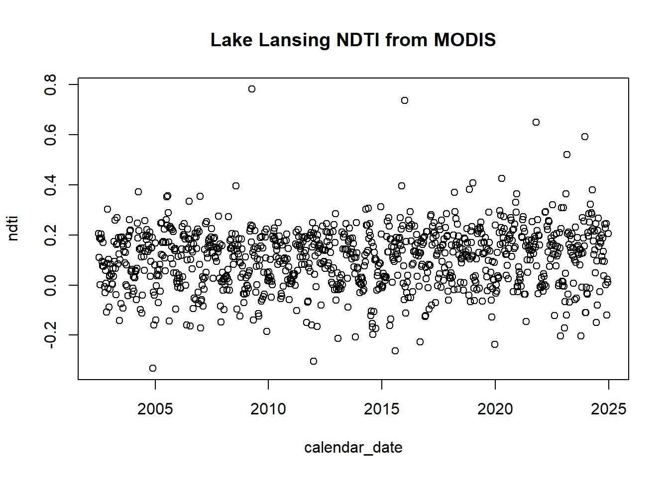
2.5 Linear Trend Analysis
As an example, I will bring in some lake data for some a random lake from some of my own work. This is median annual lake chlorophyll with some other climate and landscape variables from 1985-2018. We will focus on looking at chlorophyll alongside annual PHDI (a drought index), summer mean temperature, and total nitrogen deposition.
Run the linear models versus year (i.e., a univariate time series, no other predictors just looking for trend).
lm_chl <- lm(chl_med ~ year, data=Lake)
lm_totn <- lm(totn ~ year, data=Lake)
lm_phdi <- lm(wy_phdi_mean ~ year, data=Lake)
lm_temp <- lm(summer_tmean_mean ~ year, data=Lake)
Create plots for each of the four variables.
plot_chl <- ggplot(Lake, aes(x=year, y=chl_med)) +
  geom_point(color="blue") +
  geom_smooth(method="lm", color="red") +
  labs(title=paste("Chlorophyll micrograms/L: Slope =", round(coef(lm_chl)[2], 4),
                   ", P =", round(summary(lm_chl)$coefficients[2,4], 4))) +
  theme_minimal()

plot_totn <- ggplot(Lake, aes(x=year, y=totn)) +
  geom_point(color="blue") +
  geom_smooth(method="lm", color="red") +
  labs(title=paste("Total Nitrogen dep: Slope =", round(coef(lm_totn)[2], 4),
                   ", P =", round(summary(lm_totn)$coefficients[2,4], 4))) +
  theme_minimal()

plot_phdi <- ggplot(Lake, aes(x=year, y=wy_phdi_mean)) +
  geom_point(color="blue") +
  geom_smooth(method="lm", color="red") +
  labs(title=paste("Water Year PHDI: Slope =", round(coef(lm_phdi)[2], 4),
                   ", P =", round(summary(lm_phdi)$coefficients[2,4], 4))) +
  theme_minimal()

plot_temp <- ggplot(Lake, aes(x=year, y=summer_tmean_mean)) +
  geom_point(color="blue") +
  geom_smooth(method="lm", color="red") +
  labs(title=paste("Summer Temp C: Slope =", round(coef(lm_temp)[2], 4),
                   ", P =", round(summary(lm_temp)$coefficients[2,4], 4))) +
  theme_minimal()
grid.arrange can take our plots and arrange them into some number of columns (ncol):
## `geom_smooth()` using formula = 'y ~ x'
## `geom_smooth()` using formula = 'y ~ x'
## `geom_smooth()` using formula = 'y ~ x'
## `geom_smooth()` using formula = 'y ~ x'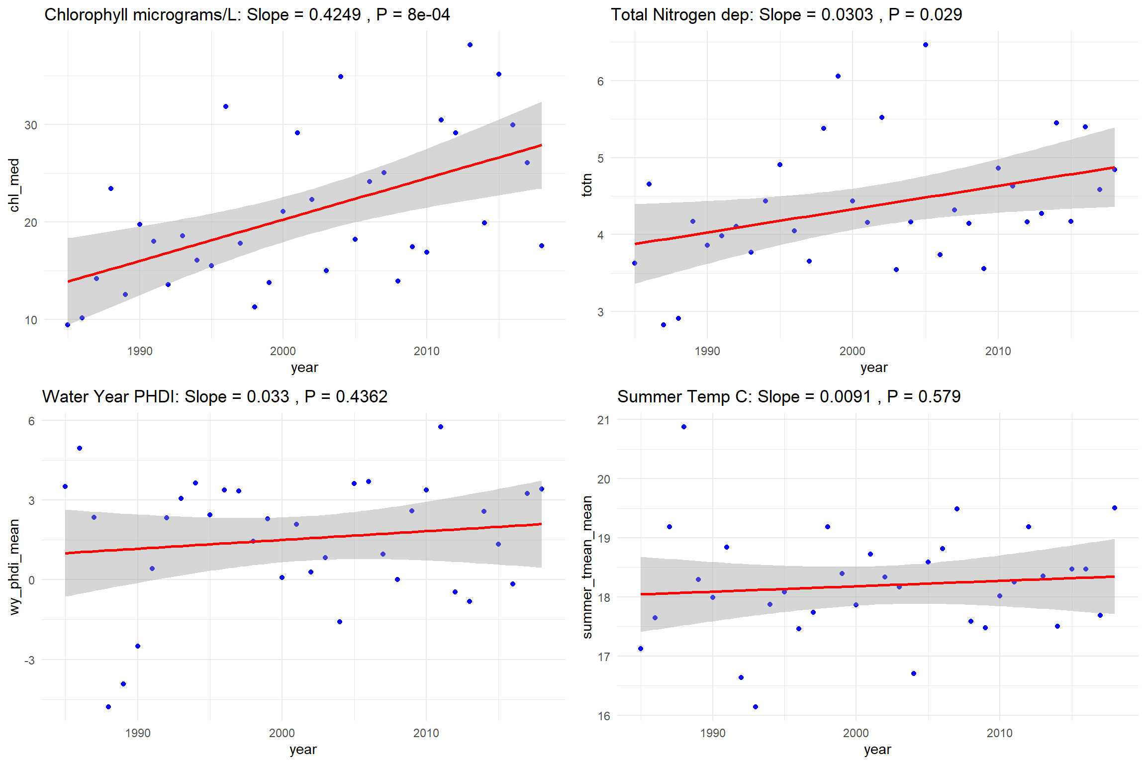
If we want to save the figure at 300 dpi as a JPEG we can do that by first initializing a jpeg of our chosen size and resolution, print our plot, and then tell it we are done with what we want to be put into the jpeg by specifying dev.off():
jpeg("lake_trend_analysis.jpeg", width=12, height=8, units="in", res=300)
grid.arrange(plot_chl, plot_totn, plot_phdi, plot_temp, ncol=2)
## `geom_smooth()` using formula = 'y ~ x'
## `geom_smooth()` using formula = 'y ~ x'
## `geom_smooth()` using formula = 'y ~ x'
## `geom_smooth()` using formula = 'y ~ x'## png
## 22.6 Mann-Kendall Trend Analysis
We run a Mann-Kendall very simply as a linear model but note that we no longer look at year since this is non-parametric and at each point the M-K test looks back at the magnitude versus each point before it. This allows it to have great flexibility for missing data, uneven sampling, etc.
mk_chl <- mk.test(Lake$chl_med)
mk_totn <- mk.test(Lake$totn)
mk_phdi <- mk.test(Lake$wy_phdi_mean)
mk_temp <- mk.test(Lake$summer_tmean_mean)Again, make the plots. This time since we don’t have a line of best fit, we will fit a LOESS (Locally Estimated Scatterplot Smoothing), which is a non-parametric regression itself and is a component of other types of non-linear time series analyses:
plot_chl <- ggplot(Lake, aes(x=year, y=chl_med)) +
geom_point(color="blue") +
geom_smooth(method="loess", color="red") +
labs(title=paste("Chlorophyll: Tau =", round(mk_chl$estimates[3], 4),
"P =", round(mk_chl$p.value, 4))) +
theme_minimal()
plot_totn <- ggplot(Lake, aes(x=year, y=totn)) +
geom_point(color="blue") +
geom_smooth(method="loess", color="red") +
labs(title=paste("Total Nitrogen: Tau =", round(mk_totn$estimates[3], 4),
"P =", round(mk_totn$p.value, 4))) +
theme_minimal()
plot_phdi <- ggplot(Lake, aes(x=year, y=wy_phdi_mean)) +
geom_point(color="blue") +
geom_smooth(method="loess", color="red") +
labs(title=paste("Water Year PHDI: Tau =", round(mk_phdi$estimates[3], 4),
"P =", round(mk_phdi$p.value, 4))) +
theme_minimal()
plot_temp <- ggplot(Lake, aes(x=year, y=summer_tmean_mean)) +
geom_point(color="blue") +
geom_smooth(method="loess", color="red") +
labs(title=paste("Summer Temp: Tau =", round(mk_temp$estimates[3], 4),
"P =", round(mk_temp$p.value, 4))) +
theme_minimal()Again plot in grid fashion with test values:
## `geom_smooth()` using formula = 'y ~ x'
## `geom_smooth()` using formula = 'y ~ x'
## `geom_smooth()` using formula = 'y ~ x'
## `geom_smooth()` using formula = 'y ~ x'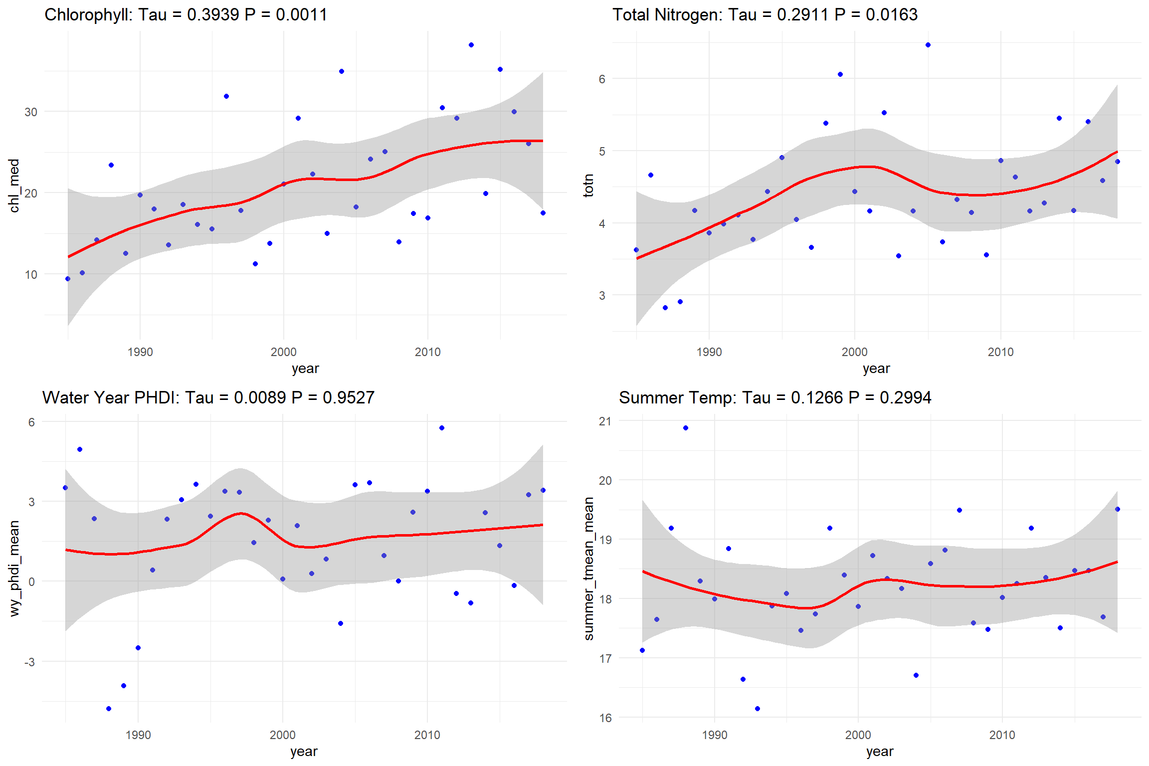
2.7 Vector Autoregressive (VAR) Model
We will run a VAR on chlorophyll to check the influence of nitrogen deposition through time.
A VAR is run on some number of lags of the variables, which can be set manually (e.g., p=2 for 2 time steps of lag) or through some automated selection process in some packages to identify the best lag. Here, I will run the VAR model for lags of 4 years:
# Select chl and totn and remove missing values
data_var <- na.omit(Lake[, c("chl_med", "totn")])

# Fit VAR models for a lag of 4
var_model <- VAR(data_var, p=4, type="both")

summary(var_model)
##
## VAR Estimation Results:
## =========================
## Endogenous variables: chl_med, totn
## Deterministic variables: both
## Sample size: 30
## Log Likelihood: -114.504
## Roots of the characteristic polynomial:
## 0.8565 0.8565 0.6861 0.6861 0.6714 0.6536 0.6536 0.4425
## Call:
## VAR(y = data_var, p = 4, type = "both")
##
##
## Estimation results for equation chl_med:
## ========================================
## chl_med = chl_med.l1 + totn.l1 + chl_med.l2 + totn.l2 + chl_med.l3 + totn.l3 + chl_med.l4 + totn.l4 + const + trend
##
## Estimate Std. Error t value Pr(>|t|)
## chl_med.l1 -0.1592 0.2248 -0.708 0.4870
## totn.l1 1.6111 2.1663 0.744 0.4657
## chl_med.l2 0.1134 0.2120 0.535 0.5986
## totn.l2 2.6514 1.7626 1.504 0.1481
## chl_med.l3 -0.2659 0.2186 -1.217 0.2379
## totn.l3 -1.2883 2.0753 -0.621 0.5418
## chl_med.l4 -0.2789 0.2546 -1.095 0.2863
## totn.l4 -3.9875 2.1781 -1.831 0.0821 .
## const 24.4716 14.3752 1.702 0.1042
## trend 0.6998 0.2691 2.600 0.0171 *
## ---
## Signif. codes: 0 '***' 0.001 '**' 0.01 '*' 0.05 '.' 0.1 ' ' 1
##
##
## Residual standard error: 6.305 on 20 degrees of freedom
## Multiple R-Squared: 0.5136, Adjusted R-squared: 0.2947
## F-statistic: 2.346 on 9 and 20 DF, p-value: 0.05387
##
##
## Estimation results for equation totn:
## =====================================
## totn = chl_med.l1 + totn.l1 + chl_med.l2 + totn.l2 + chl_med.l3 + totn.l3 + chl_med.l4 + totn.l4 + const + trend
##
## Estimate Std. Error t value Pr(>|t|)
## chl_med.l1 0.007366 0.022608 0.326 0.7479
## totn.l1 0.245678 0.217851 1.128 0.2728
## chl_med.l2 -0.035835 0.021319 -1.681 0.1083
## totn.l2 -0.410247 0.177255 -2.314 0.0314 *
## chl_med.l3 0.061265 0.021980 2.787 0.0114 *
## totn.l3 0.521453 0.208700 2.499 0.0213 *
## chl_med.l4 -0.019589 0.025601 -0.765 0.4531
## totn.l4 -0.122924 0.219045 -0.561 0.5809
## const 2.994408 1.445652 2.071 0.0515 .
## trend 0.009854 0.027064 0.364 0.7196
## ---
## Signif. codes: 0 '***' 0.001 '**' 0.01 '*' 0.05 '.' 0.1 ' ' 1
##
##
## Residual standard error: 0.6341 on 20 degrees of freedom
## Multiple R-Squared: 0.4881, Adjusted R-squared: 0.2577
## F-statistic: 2.119 on 9 and 20 DF, p-value: 0.07775
##
##
##
## Covariance matrix of residuals:
## chl_med totn
## chl_med 39.7559 -0.2124
## totn -0.2124 0.4021
##
## Correlation matrix of residuals:
## chl_med totn
## chl_med 1.00000 -0.05313
## totn -0.05313 1.00000Note in the output that a lag of 4 years means that coefficients are fit for Each of the 4 lagged periods (1, 2, 3, 4 years) for each variable, not just for 4 years.
# Extract coefficients for chl_med equation at each lag
coefficients_df <- data.frame(
  Lag = 1:4,
  Coefficient = c(var_model$varresult$chl_med$coefficients["totn.l1"],
                  var_model$varresult$chl_med$coefficients["totn.l2"],
                  var_model$varresult$chl_med$coefficients["totn.l3"],
                  var_model$varresult$chl_med$coefficients["totn.l4"]),
  P_value = c(summary(var_model$varresult$chl_med)$coefficients["totn.l1", 4],
              summary(var_model$varresult$chl_med)$coefficients["totn.l2", 4],
              summary(var_model$varresult$chl_med)$coefficients["totn.l3", 4],
              summary(var_model$varresult$chl_med)$coefficients["totn.l4", 4])
)

# Add asterisk if p-value < 0.05
coefficients_df$Label <- ifelse(coefficients_df$P_value < 0.05, "*", "")

# Convert data for plotting
coefficients_long <- melt(coefficients_df, id.vars = c("Lag", "Label"))

# Create a clean and visually appealing plot with asterisks for significance
plot_coeff <- ggplot(coefficients_long, aes(x=Lag, y=value, fill=variable)) +
  geom_bar(stat="identity", position="dodge", color="black") +
  scale_fill_manual(values=c("#1b9e77", "#d95f02")) +
  labs(title="Effect of Total Nitrogen on Chlorophyll (VAR, 4 Lags)",
       x="Lag Length", y="Coefficient Value", fill="Metric") +
  theme_minimal() +
  theme(legend.position="bottom", text=element_text(size=14)) +
  geom_text(aes(label=Label), vjust=-1, size=6, color="red") # Add asterisks above bars


# Display the plot
print(plot_coeff)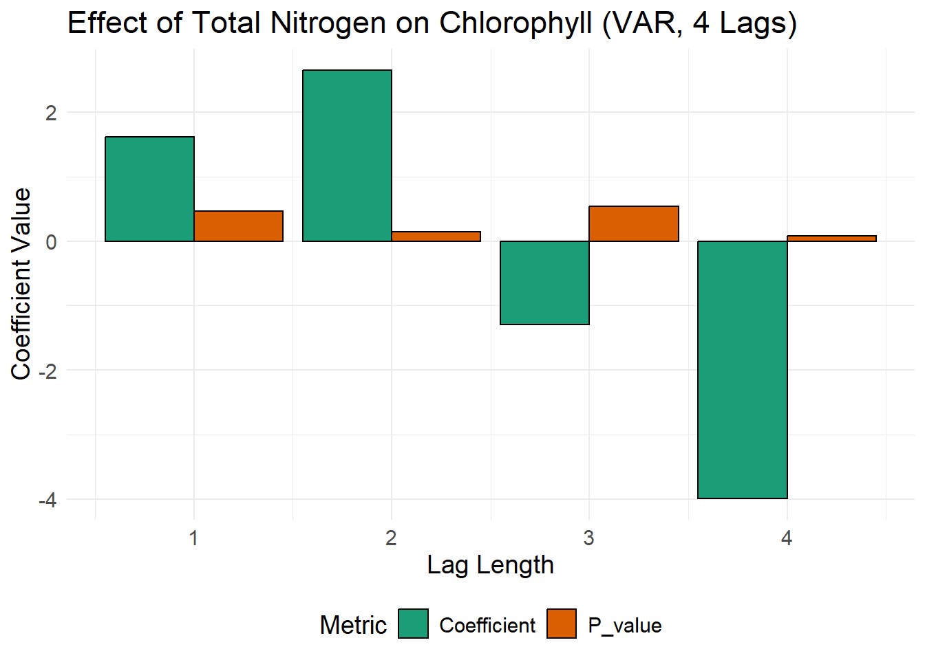
2.8 Granger Causality Analysis
Once we have the VAR model object fitted, we can see if one of those time series helps explain the others in a G-causal manner. This test can be performed in either direction (e.g., does nitrogen deposition influence chlorophyll -or- does chlorophyll influence nitrogen deposition [which would be spurious but mathematically possible]):
# Perform Granger causality tests
granger_test_1 <- causality(var_model, cause="totn")  # Testing if nitrogen Granger-causes chlorophyll
granger_test_2 <- causality(var_model, cause="chl_med")  # Testing if chlorophyll Granger-causes nitrogen

# Print results
print("Granger Causality Test: Does Total Nitrogen deposition (totn) predict Chlorophyll (chl_med)?")
## [1] "Granger Causality Test: Does Total Nitrogen deposition (totn) predict Chlorophyll (chl_med)?"##
## Granger causality H0: totn do not Granger-cause chl_med
##
## data: VAR object var_model
## F-Test = 2.3891, df1 = 4, df2 = 40, p-value = 0.06692## [1] "Granger Causality Test: Does Chlorophyll (chl_med) predict Total Nitrogen (totn)?"##
## Granger causality H0: chl_med do not Granger-cause totn
##
## data: VAR object var_model
## F-Test = 2.8207, df1 = 4, df2 = 40, p-value = 0.03751# Perform Instantaneous Causality Test
instant_causality <- causality(var_model, cause="totn")$Instant
# Print results
print("Instantaneous Causality Test: Are totn and chl_med simultaneously related?")## [1] "Instantaneous Causality Test: Are totn and chl_med simultaneously related?"##
## H0: No instantaneous causality between: totn and chl_med
##
## data: VAR object var_model
## Chi-squared = 0.084437, df = 1, p-value = 0.7714