ForSammy

Simulation

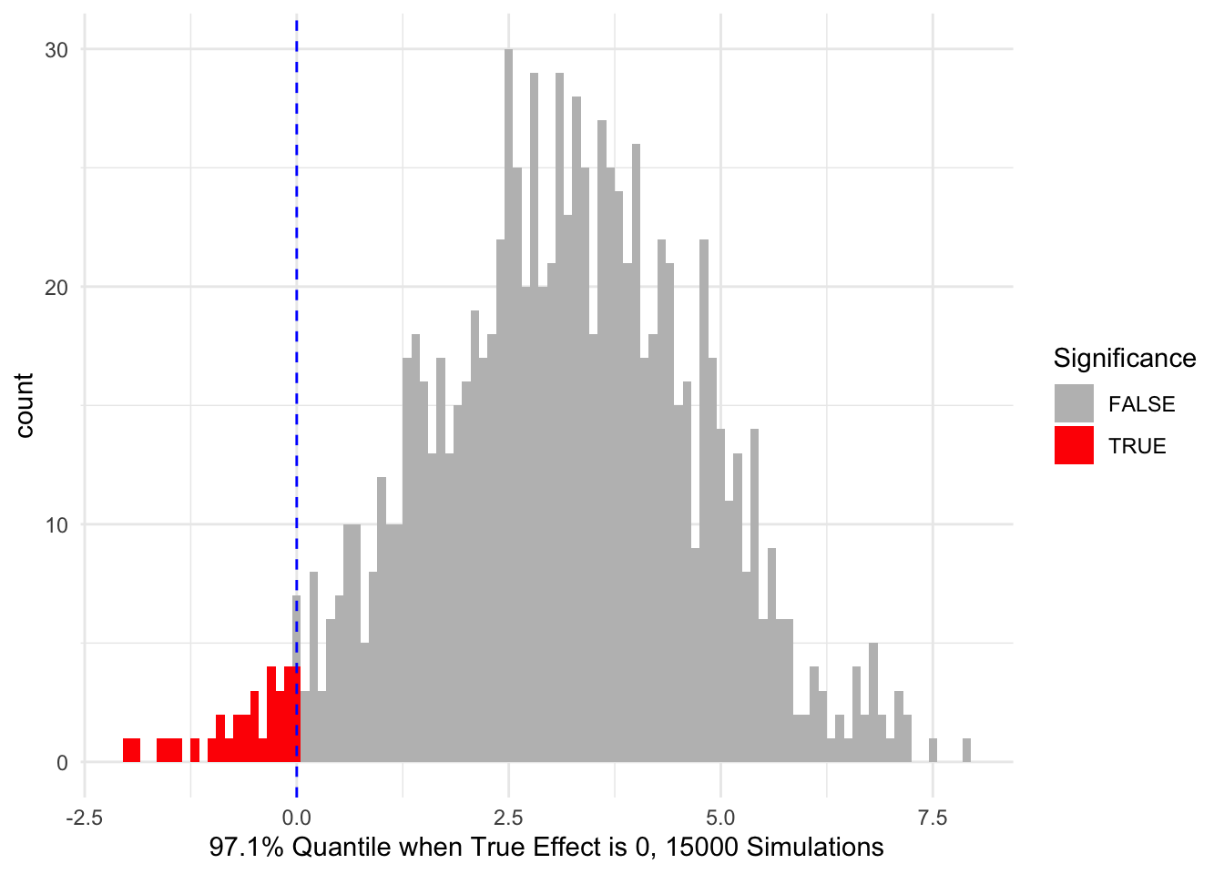
In this simulation, we are trying to understand how often our Bayesian model would falsely identify a significant effect when there is actually no effect. We set our significance threshold based on a 2.9% one-sided Type I error rate, which corresponds to the 97.1% quantile of the posterior distribution. For each simulated dataset (assuming no true effect), we fit the Bayesian model and check if the 97.1% quantile of the posterior distribution is below zero. If it is, we count it as a false positive. By repeating this process many times, we can estimate the false positive rate of our model. The histogram shows the distribution of these quantiles, with the red area indicating false positives.

Detailed Explanation

Simulation Process:

• For each simulation iteration, you generate synthetic treatment and control data assuming no true effect (both have a mean of 0).

• You fit a Bayesian model to this simulated data using prior information. Bayesian Model:

• The model uses prior distributions for treatment and control groups and updates these priors with the simulated data to obtain posterior distributions. Specifically, bdpnormal is used to fit the Bayesian model with the specified priors and data.

  Quantile Calculation

• After fitting the Bayesian model, you extract the 97.1% quantile from the posterior distribution of the treatment effect. This quantile value is used to determine if the observed effect is significant. If the 97.1% quantile is less than 0, it suggests that there is a significant effect according to your predefined threshold.

  False Positive Rate Calculation:

  If the 97.1% quantile of the posterior distribution is less than 0, it is counted as a false positive since the true effect is actually 0. You repeat this process for many simulations (n_sim), and the proportion of simulations where this occurs gives you the Type I error rate (false positive rate).

  Visualization

• Then I plot a histogram of the 97.1% quantile values from all simulations. The shaded area in red represents the proportion of simulations where the 97.1% quantile is less than 0 (false positives). The blue dashed line at 0 helps visualize how many of the quantiles fall below this threshold.

  library(bayesDP)

  Loading required package: ggplot2

  Loading required package: survival

  library(ggplot2)
  library(reshape)
  library(dplyr)

  
  Attaching package: 'dplyr'

  The following object is masked from 'package:reshape':
  
      rename

  The following objects are masked from 'package:stats':
  
      filter, lag

  The following objects are masked from 'package:base':
  
      intersect, setdiff, setequal, union

  # Function to simulate Type I error rate
  simulate_type_I_error <- function(n_sim, sample_size, treatment_sd, control_sd) {
      false_positives <- 0
      quantile_971 <- numeric(n_sim)  # Vector to store 97.1% quantiles
  
      for (i in 1:n_sim) {
          # Generate synthetic data
          treatment_data <- rnorm(sample_size / 2, 0, treatment_sd)
          control_data <- rnorm(sample_size / 2, 0, control_sd)
  
          # Fit Bayesian model
          fit <- bdpnormal(
              mu_t = mean(treatment_data), sigma_t = sd(treatment_data), N_t = sample_size / 2,
              mu0_t = -5.30, sigma0_t = 1.65 * sqrt(36), N0_t = 36,
              mu_c = mean(control_data), sigma_c = sd(control_data), N_c = sample_size / 2,
              mu0_c = -0.74, sigma0_c = 1.62 * sqrt(35), N0_c = 35,
              fix_alpha = FALSE, discount_function = "weibull", 
              weibull_scale = 0.5, weibull_shape = 3, number_mcmc = 8000
          )
  
          # Extract 97.1% quantile
          quantile_971[i] <- quantile(fit$final$posterior, probs = 0.971)
  
          # Check for false positives
          if (quantile_971[i] < 0) {
              false_positives <- false_positives + 1
          }
      }
  
      return(list(fp = false_positives / n_sim, qs = quantile_971))
  }
  
  # Run the simulation
  fpsim <- simulate_type_I_error(n_sim = 1000, sample_size = 210, treatment_sd = 12, control_sd = 12)
  
  # Plot the results
  library(ggplot2)
  data <- data.frame(qs = fpsim$qs)
  ggplot(data, aes(x = qs, fill = qs < 0)) +
    geom_histogram(binwidth = 0.1) +
    scale_fill_manual(values = c("TRUE" = "red", "FALSE" = "grey")) +
    geom_vline(xintercept = 0, color = "blue", linetype = "dashed") +
    labs(x = "97.1% Quantile when True Effect is 0, 15000 Simulations", fill = "Significance") +
    theme_minimal()