Text Analytics
2022-06-17
Session 1 Session 1
1.1 Regex Basics
Some links of interest
This link’s contents are described in what follows. http://www.regular-expressions.info/quickstart.html
This is a regex app for practice. https://regex101.com/
This is a regex primer for R in particular: http://www.regular-expressions.info/rlanguage.html
This primer’s objective is only to learn as much regex as we need for what follows.
Students are encouraged to explore the links above as a starting point for any deeper study.
1.1.1 Metacharacters
Twelve characters have special meanings in regular expressions:
the backslash
\- escape character for literal reading of metacharacters (see below for examples)the caret
^- matches at the start of the string; negates a character class (see below for examples)the dollar sign
$- matches at the end of the stringthe period or dot
.- matches ANY character (except the newline)the vertical bar or pipe symbol
|- OR logic gatethe question mark
?- evaluates if a character class existsthe asterisk or star
*- zero or more occurrences/ repetitionsthe plus sign
+- one or more matches/repetitionsthe opening parenthesis
(the closing parenthesis
)- these enclose a character set togetherthe opening square bracket
[the opening curly brace
{- number of repetitions can be precisely specified
These special characters are often called “metacharacters”. Most of them are errors when used alone.
If you want to use any of these characters as a literal in a regex, you need to escape them with a backslash.
E.g., to match 1+1=2, the correct regex is 1\+1=2.
You escape a backslash by using another backslash. E.g., \\s
1.1.2 Character Class
A “character class” matches only one out of several characters.
Use a hyphen inside a character class to specify a range of characters. E.g., [0-9] matches a single digit between 0 and 9.
Typing a caret (^) after the opening square bracket negates the character class. E.g., [^0-9] matches any character except numeric digits.
1.1.3 Shorthand Character Classes
\\d matches a single character that is a digit,
\\w matches a “word character” (alphanumeric characters plus underscore), and
\\s matches a whitespace character (includes tabs and line breaks).
\\t matches a tab character (ASCII 0x09),
\\r carriage return (0x0D) and
\\nfor line feed (0x0A).
The dot matches a single character, except line-break characters.
1.1.4 Anchors
Anchors do not match any characters. They match a position.
^ matches at the start of the string, and $ matches at the end of the string.
E.g. ^b matches only the first b in bob.
\\b matches at a word boundary. A word boundary is a position between a character that can be matched by \\w and a character that cannot be matched by \\w.
1.1.5 Alternation
Alternation is the regular expression equivalent of “or”. E.g., cat|dog matches cat in About cats and dogs.
Alternation has the lowest precedence of all regex operators. cat|dog food matches cat or dog food.
To create a regex that matches cat food or dog food, you need to group the alternatives: (cat|dog) food.
1.1.6 Repetition
The question mark makes the preceding token in the regular expression optional. E.g., colou?r matches colour or color.
The asterisk or star tells the engine to attempt to match the preceding token zero or more times.
The plus tells the engine to attempt to match the preceding token once or more.
E.g., <[A-Za-z][A-Za-z0-9]*> matches an HTML tag without any attributes. <[A-Za-z0-9]+> is easier to write but matches invalid tags such as <1>.
Use curly braces to specify a specific amount of repetition.
E.g., Use \\b[1-9][0-9]{3}\\b to match a number between 1000 and 9999.
\\b[1-9][0-9]{2,4}\\b matches a number between 100 and 99999.
1.2 Regex Exercise
How about a quick exercise, eh?
Go to https://regex101.com/
Now copy-paste the text below into the regex app.
ISB has been ranked 27th in the world in the 2017 Financial Times Global MBA Rankings.[3] It is the first business school in Indian subcontinent to be accredited by the Association to Advance Collegiate Schools of Business.[4] In 2008, it became the youngest institution to find a place in global MBA rankings when it was ranked 20.[5] Indian School of Business accepts both GMAT and GRE scores for the admission process.
This is an exclamatory sentence!! Is this one an interrogative one?? This one has an ellipsis… And this is a declarative sentence. My phone number is 12345 67890 whereas that of the school is +91-040-2318-7000.
1.3 Tokenization from First Principles
1.3.1 Introduction
Tokenization is the process of breaking down written text into distinct units of analysis - typically words.
However the process of breaking down text into units of analysis also extends to both a smaller scale such as at the character or syllable level, or a larger scale such as combinations of words (n-grams), chunks of words (e.g., phrases), larger units such as sentences and paragraphs etc (at which point, it becomes parsing).
In what follows, we use functions from the the stringr package to construct a simple tokenizer.
First load the libraries we need
suppressPackageStartupMessages({
  if (! require(stringr)){install.packages("stringr", dependencies = TRUE)}
  library(stringr)
})
The plan is to start with tokenizing on a single, simple sentence. We’ll then extend it to larger collections of sentences.
1.3.2 Some basic string ops
# Example Commands
  my_string <- "My PHONE number is +91 40 2318 7106, is it?!"
  my_string
## [1] "My PHONE number is +91 40 2318 7106, is it?!"lower_string <- tolower(my_string) # makes lower case
lower_string## [1] "my phone number is +91 40 2318 7106, is it?!"second_string <- "OK folks, Second sentence, coming up."; second_string## [1] "OK folks, Second sentence, coming up."my_string <- paste(my_string, # try `?paste`
second_string,
sep = " ")
my_string## [1] "My PHONE number is +91 40 2318 7106, is it?! OK folks, Second sentence, coming up."So far, so good. Let’s start splitting the strings next.
# Now, split out string up into a number of strings using the str_split() func
  my_string_vector <- str_split(my_string, "!")[[1]]

  my_string_vector
## [1] "My PHONE number is +91 40 2318 7106, is it?"
## [2] " OK folks, Second sentence, coming up."Notice in my_string_vectcor above, that the splitting character (“!”) gets deleted and a list object is returned. Hence, the use of the list operator ([[1]]) to get the first entry.
In what follows, we’ll see the following functions in action. grep() and grepl() to find a particular text pattern using regex if necessary. We also have str_replace_all and str_extract_all coming up.
# search for string in my_string_vector that contains a `?` using the `grep()` command
  grep("\\?", my_string_vector)    # gives location of vector that contains match
## [1] 1# using a conditional statement with logical grep, `grepl()`, maybe useful
grepl("\\?", my_string_vector[1]) # logical grep() for binary T/F output## [1] TRUE# str_replace_all() func replaces all instances of some characters with another character
str_replace_all(my_string, "e","___")## [1] "My PHONE numb___r is +91 40 2318 7106, is it?! OK folks, S___cond s___nt___nc___, coming up."# using regex to extract all numbers from a string
str_extract_all(my_string, "[0-9]+") # doesn't match decimals though## [[1]]
## [1] "91" "40" "2318" "7106"# alternately
str_extract_all(my_string, "[^a-zA-Z\\s]+") # every char not in a-z, A-Z or space \\s## [[1]]
## [1] "+91" "40" "2318" "7106," "?!" "," "," "." str_extract_all(my_string, "[\\d]+") # every char that is a digit## [[1]]
## [1] "91" "40" "2318" "7106"OK, finally. Let’s write our first, simple tokenizer.
1.3.3 A Simple Word Tokenizer
# string split taking space as token-separator.
tokenized_vec = str_split(my_string, "\\s")

# basic tokenization using spaces
tokenized_vec
## [[1]]
## [1] "My" "PHONE" "number" "is" "+91" "40"
## [7] "2318" "7106," "is" "it?!" "OK" "folks,"
## [13] "Second" "sentence," "coming" "up."We now know that with the appropriate regex expressions, we can narrow the above down to only include words and get rid of the numbers.
1.3.4 Functionizing the Tokenizer Workflow
Given what we have seen above, next, how about we functionize (so to say) what we did above?
If we write a function that automates the steps above, we could repeatedly invoke the function wherever required.
That’s where we are going next. I’ll define a simple func called clean_string() (note naming convention for funcs) that will pre-process messy input text.
## Cleaning Text and Tokenization from First Principles (using Regex) ##

  clean_string <- function(string){

    require(stringr)

    temp <- tolower(string)   # Lowercase

    # Replace all non-alpha-numerics with space
    temp <- stringr::str_replace_all(temp,"[^a-zA-Z\\s]", " ")

    # collapse one or more spaces into one space using `+` regex or for repeats >1
    temp <- stringr::str_replace_all(temp,"[\\s]+", " ")

    # Split string using space as separator
    temp <- stringr::str_split(temp, " ")[[1]]

    # Get rid of trailing "" if necessary
    indexes <- which(temp == "")

    if(length(indexes) > 0){ temp <- temp[-indexes] }

    return(temp)

  } # Clean_String func ends
Everyone with me so far? Go line-by-line later and ensure everything there is clear!
Now, let’s apply the function to a simple example and see.
Below is a line from Shakespere’s As you like it.
sentence <- "All the world's a stage, and all the men and women merely players: they have their exits and their entrances; and one man in his time plays many parts.' "

  clean_sentence <- clean_string(sentence)   # invoking the function
  print(clean_sentence)   # view func output
## [1] "all" "the" "world" "s" "a" "stage"
## [7] "and" "all" "the" "men" "and" "women"
## [13] "merely" "players" "they" "have" "their" "exits"
## [19] "and" "their" "entrances" "and" "one" "man"
## [25] "in" "his" "time" "plays" "many" "parts" unique(clean_sentence) # de-duplicated version using `unique()`.## [1] "all" "the" "world" "s" "a" "stage"
## [7] "and" "men" "women" "merely" "players" "they"
## [13] "have" "their" "exits" "entrances" "one" "man"
## [19] "in" "his" "time" "plays" "many" "parts"While the above was neat and all, it was still just one sentence. But what about large corpora with many, many documents, each with many, many sentences?
What we can do next is to use the above function as a subroutine in a larger function that will loop over sentences in documents. See the code below.
 ## === Now extend to multiple documents. Function to clean text blocks (or corpora)

  clean_text_block <- function(text){

      # Check to see if there is any text at all with another conditional
      if(length(text) == 0){ cat("There was no text in this document! \n"); stop }

      # Get rid of blank lines
      indexes <- which(text == "")
      if(length(indexes) > 0){ text <- text[-indexes]   }

      # Loop through the lines in the text and use the `append()` function
      clean_text <- clean_string(text[1])

      if (length(text)>1){

        for(i in 2:length(text)){

        # add them to a vector
        clean_text <- append(clean_text, clean_string(text[i])) }   # i loop ends

            } # if condn ends

      # Calc number of tokens and unique tokens. Return them in a named list object.
      num_tok <- length(clean_text)
      num_uniq <- length(unique(clean_text))

      to_return <- list(num_tokens = num_tok,   # output is list with 3 elements
                        unique_tokens = num_uniq,
                        text = clean_text)

    return(to_return)   } # clean_text_block() func ends
Now, let’s try it on a sizeable dataset.
1.3.5 Tokenizing a real world dataset
The Amazon Nokia Lumia reviews dataset is an old dataset with about 120 consumer reviews. Not too large and will do for our purposes.
You can either read the file in using readLines(file.choose()) or directly read it off my Github page.
 text <- readLines('https://github.com/sudhir-voleti/sample-data-sets/raw/master/text%20analysis%20data/amazon%20nokia%20lumia%20reviews.txt')

  system.time({
    clean_speech <- clean_text_block(text[1:10])   # invoking the func
    })    # didn't take long now, did it?
## user system elapsed
## 0.022 0.004 0.027 str(clean_speech) # unlist and view structure of the output## List of 3
## $ num_tokens : int 2831
## $ unique_tokens: int 786
## $ text : chr [1:2831] "i" "have" "had" "samsung" ... clean_speech$text[1:40] # view first 40 tokens from the dataset## [1] "i" "have" "had" "samsung" "phones" "where"
## [7] "the" "screens" "are" "nice" "but" "the"
## [13] "plastic" "bodies" "come" "apart" "all" "of"
## [19] "the" "time" "and" "feel" "flimsy" "i"
## [25] "have" "had" "iphones" "where" "the" "user"
## [31] "interface" "is" "just" "so" "boring" "even"
## [37] "with" "all" "those" "apps"With basic tokenization done, we can now proceed and, from first principles alone, build a lot of text analysis functionality.
However, that would be duplicating a lot of work already done in R. There are many excellent packages in R that do the above - tokenizing etc and thereafter building data structures for further analysis.
We will follow that route. But it is important to know that, if need be, we could build all that functionality from first principles if we wanted to.
Sudhir Voleti
1.4 Introductory Text An with Tidy-Text
1.4.1 Basic Intro to Tidytext
Tidytext is text-an part of ‘tidyverse’ - a set of popular packages that work on a common set of code principles called the ‘tidy data framework’ originally created by the legendary (in R circles, at least) Hadley Wickham.
We’ll see some of these tidy data handling procedures as we proceed ahead. Tidytext (Silge and Robinson 2016) is described thus by its creators:
“Treating text as data frames of individual words allows us to manipulate, summarize, and visualize the characteristics of text easily and integrate natural language processing into effective workflows we were already using.”
So let’s jump right in.
suppressPackageStartupMessages({
if (!require(tidyverse)) {install.packages("tidyverse")}
if (!require(tidytext)) {install.packages("tidytext")}

library(tidyverse)
library(tidytext)
library(ggplot2)
})
1.4.2 Tidytext Analysis on the Nokia dataset
I return to an old favorite here: the 2013 Amazon Nokia Lumia reviews dataset of 120 consumer reviews.
For this example, we can read the data directly off my github page. Behold.
# Example reading in an amazon nokia corpus
nokia = readLines('https://github.com/sudhir-voleti/sample-data-sets/raw/master/text%20analysis%20data/amazon%20nokia%20lumia%20reviews.txt')

text <- nokia
text  =  gsub("<.*?>", " ", text)              # regex for removing HTML tags
length(text)    # 120 documents
## [1] 1201.4.3 Tidytext Tokenization with unnest_tokens()
First thing to note before invoking tidytext - get the text into a data_frame format, called a tibble, which has nice printing properties - e.g., it never floods the console.
In other words, we convert text_df into one-token-per-document-per-row.
Now time to see tidytext’s neat tokenizing capabilities at the level of:
- words,
- sentences,
- paragraphs, and
- ngrams,
using the unnest_tokens() function.
require(tibble)
textdf = tibble(text = text) # yields 120x1 tibble. i.e., each doc = 1 row here.

textdf # view the tibble DF obj
## # A tibble: 120 × 1
## text
## <chr>
## 1 "I have had Samsung phones, where the screens are nice, but the plastic bodi…
## 2 "This phone is great! It's the best phone I've ever owned. I have been a ded…
## 3 "I just bought this phone a few weeks ago and it is gorgeous. The screen jus…
## 4 "Hi, I bought a cell phone by Amazon with the following description: \"Noki…
## 5 "The Nokia Lumia 900 was my first smartphone. Im a programmer, so I really a…
## 6 "I am a tmobile customer and with an unlocked Nokia 900 Lumia from ATT .Let …
## 7 "I bought this phone because I wanted to use it on TMobile. I've only been f…
## 8 "I received my phone before the expected arrival date and in excellent condi…
## 9 "I bought the phone and it was nice but has one problem that my husband did …
## 10 "I purchased the Nokia Lumina 900 in black from BLUTECUSA and was really thr…
## # … with 110 more rows# Tokenizing ops. Words first.
system.time({
textdf %>% unnest_tokens(word, text) # try ?unnest_tokens
})## user system elapsed
## 0.006 0.000 0.007So, how many words are there in the Nokia corpus?
Below, we can see sentence tokenization using the token = "sentences" parm in unnest_tokens.
# Tokenizing into sentences.
system.time({
  sent_tokenized = textdf %>%
    unnest_tokens(sentence, text, token = "sentences") # 905 rows/120 docs ~8 sents per doc?
  })   # 0 secs
## user system elapsed
## 0.003 0.000 0.003# explore output object a bit
class(sent_tokenized)## [1] "tbl_df" "tbl" "data.frame"dim(sent_tokenized)## [1] 905 1head(sent_tokenized)## # A tibble: 6 × 1
## sentence
## <chr>
## 1 i have had samsung phones, where the screens are nice, but the plastic bodies…
## 2 i have had iphones, where the user interface is just so boring, even with all…
## 3 the nokia has wonderful nokia apps already installed, such as nokia drive, wh…
## 4 you get nokia music, which is a free music service with 1500 playlists put to…
## 5 you get espn, nokia city lens, which is where you hold your camera up while y…
## 6 and there are other free nokia apps as well, like camera extras, that let you…Sentence detection appears to be good, above.
Tokenizing DF into bigrams, below. Try different ngrams & see.
system.time({
  ngram_tokenized = textdf %>%
    unnest_tokens(ngram, text, token = "ngrams", n = 2) # yields (#tokens-1) bigrams
  })  # 0.03 secs
## user system elapsed
## 0.007 0.000 0.008#explore the output object
class(ngram_tokenized)## [1] "tbl_df" "tbl" "data.frame"dim(ngram_tokenized)## [1] 15275 1head(ngram_tokenized)## # A tibble: 6 × 1
## ngram
## <chr>
## 1 i have
## 2 have had
## 3 had samsung
## 4 samsung phones
## 5 phones where
## 6 where the1.4.4 Grouping, Aggegation and Join ops in tidytext
Intuitively, the funcs we’ll call in tidytext are named group_by(), count() and join(). Behold.
# use count() to see most common words
system.time({
nokia_words = textdf %>%
        unnest_tokens(word, text) %>%  # tokenized words in df in 'word' colm
        count(word, sort = TRUE) %>%   # counts & sorts no. of occurrences of each item in 'word' column
        rename(count = n)      # renames the count column from 'n' (default name) to 'count'.
  }) # 0.11 secs
## user system elapsed
## 0.037 0.000 0.037nokia_words %>% head(., 10) # view top 10 rows in nokia-words df## # A tibble: 10 × 2
## word count
## <chr> <int>
## 1 the 682
## 2 i 510
## 3 and 448
## 4 to 427
## 5 phone 388
## 6 a 362
## 7 it 358
## 8 is 299
## 9 for 202
## 10 this 201Unsurprisingly, the most common words, with the highest no. of occurrences are the scaffolding of grammer - articles, prepositions, conjunctions etc. Not exactly the meaty stuff.
Is there anything we can do about it? Yes, we can. (Pun intended). We could filter the words using a stopwords list from earlier.
Conveniently, tidytext comes with its own stop_words list.
data(stop_words)

# use anti_join() to de-merge stopwords from the df
system.time({

  nokia_new = textdf %>%
        unnest_tokens(word, text) %>%
        count(word, sort = TRUE) %>%
        rename(count = n) %>%
        anti_join(stop_words)   # try ?anti_join

  })  # 0.03 secs
## Joining, by = "word"## user system elapsed
## 0.044 0.000 0.045 nokia_new %>% head(., 10)## # A tibble: 10 × 2
## word count
## <chr> <int>
## 1 phone 388
## 2 nokia 87
## 3 windows 77
## 4 apps 70
## 5 lumia 62
## 6 900 45
## 7 unlocked 45
## 8 phones 42
## 9 battery 34
## 10 android 32Aha. With the stopwords filtered out, the scene changes quite a bit.
How about some visualization via bar-charts, just for completeness? See below.
# First, build a datafame
tidy_nokia <- textdf %>%
  unnest_tokens(word, text) %>%     # word tokenization
  anti_join(stop_words)    # run ?join::dplyr
## Joining, by = "word"# Visualize the commonly used words using ggplot2.
library(ggplot2)
tidy_nokia %>%
count(word, sort = TRUE) %>%
filter(n > 20) %>% # n is wordcount colname.
mutate(word = reorder(word, n)) %>% # mutate() reorders columns & renames too
ggplot(aes(word, n)) +
geom_bar(stat = "identity", col = "red", fill = "red") +
xlab(NULL) +
coord_flip()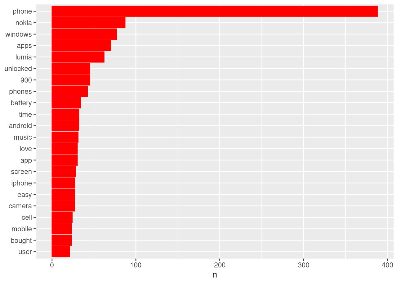 ### More Bigram ops with tidytext
Bigrams in particular, and ngrams in general will have several uses down the line, as we’ll see. As such they link BOW with NLP in a way.
First, let’s build and view the bigrams with token = "ngrams, n=2 argument in the unnest_tokens() func.
nokia_bigrams <- textdf %>%
  unnest_tokens(bigram, text,
                token = "ngrams", n = 2)
nokia_bigrams
## # A tibble: 15,275 × 1
## bigram
## <chr>
## 1 i have
## 2 have had
## 3 had samsung
## 4 samsung phones
## 5 phones where
## 6 where the
## 7 the screens
## 8 screens are
## 9 are nice
## 10 nice but
## # … with 15,265 more rowsNow use separate() to str_split() the words.
require(tidyr)
# separate bigrams
bigrams_separated <- nokia_bigrams %>%
                        separate(bigram, c("word1", "word2"), sep = " ")
bigrams_separated
## # A tibble: 15,275 × 2
## word1 word2
## <chr> <chr>
## 1 i have
## 2 have had
## 3 had samsung
## 4 samsung phones
## 5 phones where
## 6 where the
## 7 the screens
## 8 screens are
## 9 are nice
## 10 nice but
## # … with 15,265 more rowsVery many stopwords in there obscuring meaning. So let’s remove them by successively doing filter() on the first and second words.
# filtering the bigrams to remove stopwords
bigrams_filtered <- bigrams_separated %>%
                      filter(!word1 %in% stop_words$word) %>%
                      filter(!word2 %in% stop_words$word)

bigrams_filtered
## # A tibble: 1,969 × 2
## word1 word2
## <chr> <chr>
## 1 samsung phones
## 2 plastic bodies
## 3 feel flimsy
## 4 user interface
## 5 wonderful nokia
## 6 nokia apps
## 7 nokia drive
## 8 talking attendant
## 9 super accurate
## 10 nokia music
## # … with 1,959 more rowsOther ops like counting and sorting should be standard by now.
# New bigram counts:
bigram_counts <- bigrams_filtered %>%
        count(word1, word2, sort = TRUE)

bigram_counts
## # A tibble: 1,631 × 3
## word1 word2 n
## <chr> <chr> <int>
## 1 lumia 900 34
## 2 windows phone 31
## 3 nokia lumia 23
## 4 battery life 14
## 5 cell phone 12
## 6 lumia 920 12
## 7 sim card 12
## 8 windows 8 11
## 9 data plan 7
## 10 gorilla glass 7
## # … with 1,621 more rowstidyr’s unite() function is the inverse of separate(), and lets us recombine the columns into one.
Thus, “separate / filter / count / unite” functions let us find the most common bigrams not containing stop-words.
bigrams_united <- bigrams_filtered %>%
  unite(bigram, word1, word2, sep = " ")
bigrams_united
## # A tibble: 1,969 × 1
## bigram
## <chr>
## 1 samsung phones
## 2 plastic bodies
## 3 feel flimsy
## 4 user interface
## 5 wonderful nokia
## 6 nokia apps
## 7 nokia drive
## 8 talking attendant
## 9 super accurate
## 10 nokia music
## # … with 1,959 more rowsSuppose we want to identify all those bigrams wherein the words “cloud”, “windows” or “solution” appeared either in word1 or in word2.
In other words, we want to match arbitrary word strings with bigram components. See code below.
# filter for bigrams which contain the word game, intelligent, or cloud
arbit_filter = bigrams_filtered %>%
            filter(word1 %in% c("windows", "solution", "cloud") | word2 %in% c("windows", "solution", "cloud")) %>%
      count(word1, word2, sort = TRUE)

arbit_filter %>% filter(word1 == "windows" | word2 == "cloud")   # try for cloud in word2 etc.
## # A tibble: 22 × 3
## word1 word2 n
## <chr> <chr> <int>
## 1 windows phone 31
## 2 windows 8 11
## 3 windows phones 7
## 4 windows 7.5 3
## 5 windows platform 3
## 6 windows 7 2
## 7 windows 7.8 2
## 8 windows live 2
## 9 free cloud 1
## 10 frees cloud 1
## # … with 12 more rows1.4.5 Casting tidy data into DTMs
Nice that tidy data can do so much. But how about building standard text-an data objects like DTMs etc?
Sure, tidytext can very well do that. First, we convert the text corpus into the tidy format, essentially, one-token-per-row-per-document. See the code below.
# First convert Nokia corpus to tidy format, i.e. a tibble with token and count per row per document.

tidy_nokia = textdf %>%
                    mutate(doc = row_number()) %>%
                    unnest_tokens(word, text) %>%
                    anti_join(stop_words) %>%
                    group_by(doc) %>%
                    count(word, sort=TRUE)
## Joining, by = "word"tidy_nokia## # A tibble: 4,196 × 3
## # Groups: doc [120]
## doc word n
## <int> <chr> <int>
## 1 25 phone 27
## 2 59 lumia 20
## 3 2 phone 15
## 4 19 phone 12
## 5 8 phone 11
## 6 25 sms 11
## 7 25 view 11
## 8 59 920 11
## 9 59 windows 11
## 10 25 option 10
## # … with 4,186 more rowsNow, to cast this tidy object into a DTM, into a regular (if sparse) matrix etc. See code below.
# cast into a Document-Term Matrix
nokia_dtm = tidy_nokia %>%
            cast_dtm(doc, word, n)

nokia_dtm   # yields a sparse matrix format by default
## <<DocumentTermMatrix (documents: 120, terms: 1964)>>
## Non-/sparse entries: 4196/231484
## Sparsity : 98%
## Maximal term length: 17
## Weighting : term frequency (tf)Below, we convert tidy_nokia into a regular matrix.
# cast into a Matrix object
nokia_dtm <- tidy_nokia %>% cast_sparse(doc, word, n)
    # class(nokia_dtm)  # Matrix

nokia_dtm[1:6,1:6]
## 6 x 6 sparse Matrix of class "dgCMatrix"
## phone lumia sms view 920 windows
## 25 27 7 11 11 . 1
## 59 9 20 . . 11 11
## 2 15 2 . . . 4
## 19 12 1 . . . 5
## 8 11 2 . . . 2
## 9 9 . . . . .1.4.6 the TFIDF transformation
Recall we mentioned there’re two weighing schemes for token frequencies in the DTM.
What we saw above was the simpler, first one, namely, term frequency or TF.
Now we introduce the second one - TFIDF. Which stands for term frequency-inverse document frequency.
Time to move to the slides and the board before returning here. Tidytext code for the TFIDF transformation is below.
P.S. Let \(tf(term)\) denote the term frequncy of some term of interest. Then \(tfidf(term)\) is defind as \(\frac{tf(term)}{idf(term)}\)
where \(idf(term) = ln\frac{n_{documents}}{n_{documents.with.term}}\). Various other schemes have been proposed.
 nokia_dtm_idf = tidy_nokia %>%
        group_by(doc) %>%
        count(word, sort=TRUE) %>% ungroup() %>%
        bind_tf_idf(word, doc, n) %>%
        cast_sparse(doc, word, tf_idf)

 nokia_dtm_idf[1:8, 1:8]   # view a few rows
## 8 x 8 sparse Matrix of class "dgCMatrix"
## 1080p 1500 7.5 720p 7gb accurate action
## 1 0.03198707 0.03740228 0.02482855 0.03740228 0.03198707 0.03740228 0.03740228
## 2 . . . . 0.03411954 . .
## 3 . . . . . . .
## 4 . . . . . . .
## 5 . . . . . . .
## 6 . . . . . . .
## 7 . . . . . . .
## 8 . . . . . . .
## adjust
## 1 0.03198707
## 2 .
## 3 .
## 4 .
## 5 .
## 6 .
## 7 .
## 8 .Last but not least is the ability to explicitly leverage tidytext’s tidy data format to do some cool stuff. Below is only if we have time.
1.4.7 Applying Tidy Principles on Text data
The Nokia corpus has 120 documents. Each document has several sentences. And each sentence has several words in it. Here’s a Q for you now.
Suppose you want to know how many sentences are there in each document in the corpus. And how many words are there in each sentence. How would you go about this?
dplyr functions inside tidytext get us there easily because the data are arranged as per tidy principles.
I present a few simple examples below. These operators while simple enable us to build fairly complex structures by recombining and chaining them together.
Let’s answer the question set above. I’ll use functions row_number() and group_by(). See the code below.
### Create a document id and group_by it
textdf_doc = textdf %>%
              mutate(doc = row_number()) %>%   # creates an id number for each row, i.e., doc.
              select(doc, text)
              # group_by(doc)   # internally groups docs together

textdf_doc
## # A tibble: 120 × 2
## doc text
## <int> <chr>
## 1 1 "I have had Samsung phones, where the screens are nice, but the plasti…
## 2 2 "This phone is great! It's the best phone I've ever owned. I have been…
## 3 3 "I just bought this phone a few weeks ago and it is gorgeous. The scre…
## 4 4 "Hi, I bought a cell phone by Amazon with the following description: …
## 5 5 "The Nokia Lumia 900 was my first smartphone. Im a programmer, so I re…
## 6 6 "I am a tmobile customer and with an unlocked Nokia 900 Lumia from ATT…
## 7 7 "I bought this phone because I wanted to use it on TMobile. I've only …
## 8 8 "I received my phone before the expected arrival date and in excellent…
## 9 9 "I bought the phone and it was nice but has one problem that my husban…
## 10 10 "I purchased the Nokia Lumina 900 in black from BLUTECUSA and was real…
## # … with 110 more rowsSo I have doc id and corresponding text. What I next need is a sentence identifier within each doc.
Then, a word identifier for each word within each sentence. Finally, can simply merge the dataframes. See below.
### How many sentences in each doc?
textdf_sent = textdf_doc %>%
              unnest_tokens(sentence, text, token = "sentences") %>%

              group_by(doc) %>%
              mutate(sent_id = row_number()) %>%      # create sentence id by enumeration
              summarise(sent_doc = max(sent_id)) %>%  # max sent_id is the num of sents in doc

              select(doc, sent_doc)    # retain colms in order for clean display

textdf_sent   # first few rows, view.
## # A tibble: 120 × 2
## doc sent_doc
## <int> <int>
## 1 1 17
## 2 2 28
## 3 3 21
## 4 4 6
## 5 5 19
## 6 6 27
## 7 7 5
## 8 8 25
## 9 9 7
## 10 10 4
## # … with 110 more rowsSo, on average how many sentences does a product reviewer write on Amazon for this corpus? The above DF gives the answer.
Next, to find average doc length, will need to know how many words are there in each document. See below.
### How many words in each document?
textdf_word = textdf_doc %>%   # using textdf_doc and not textdf_sent!
              unnest_tokens(word, text) %>%

              group_by(doc) %>%
              mutate(word_id = row_number()) %>%
              summarise(word_doc = max(word_id)) %>%
              select(doc, word_doc)

textdf_word[1:10,]
## # A tibble: 10 × 2
## doc word_doc
## <int> <int>
## 1 1 415
## 2 2 521
## 3 3 322
## 4 4 92
## 5 5 348
## 6 6 459
## 7 7 65
## 8 8 336
## 9 9 164
## 10 10 58The Qs continue. So I have textdf_sent that maps sentences to documents and textdf_word that maps wordcounts to document.
Can I combine the two dataframes? Yes we can. Try ?inner_join and see.
### can we merge the above 2 tables together?
# colnames(textdf_sent)   # doc, sent_doc
# colnames(textdf_word)   # doc, word_doc

doc_sent_word = inner_join(textdf_sent,   # first df
                           textdf_word,   # second df
                           by = "doc") %>% # inner_join by 'doc' colm

                      mutate(words_per_sent = word_doc/sent_doc)   # avg no. of words per sentence as a new variable

doc_sent_word[1:10,]   # view first few rows of the new merged table
## # A tibble: 10 × 4
## doc sent_doc word_doc words_per_sent
## <int> <int> <int> <dbl>
## 1 1 17 415 24.4
## 2 2 28 521 18.6
## 3 3 21 322 15.3
## 4 4 6 92 15.3
## 5 5 19 348 18.3
## 6 6 27 459 17
## 7 7 5 65 13
## 8 8 25 336 13.4
## 9 9 7 164 23.4
## 10 10 4 58 14.5Neat, eh? One last thing. We’ve mapped sentences to documents and words to docs. Can we now map words to sentences?
In other words, how many words are there per sentence? See below.
### how many words in each sentence?
textdf_sent_word = textdf %>%
                    unnest_tokens(sentence, text, token = "sentences") %>%
                    mutate(senten = row_number()) %>% # building an index for sentences now
                    select(senten, sentence) %>%

                          unnest_tokens(word, sentence) %>%
                    mutate(word_id = row_number()) %>%   # creating an intermed variable for word-counting
                    select(senten, word_id) %>%

                          group_by(senten) %>%  # grouping by sent id
                    summarise(words_in_sent = max(word_id)) %>% # summarizing
                    select(senten, words_in_sent)       # retain only relevant cols

textdf_sent_word[11:20,]
## # A tibble: 10 × 2
## senten words_in_sent
## <int> <int>
## 1 11 301
## 2 12 319
## 3 13 340
## 4 14 373
## 5 15 392
## 6 16 407
## 7 17 415
## 8 18 419
## 9 19 426
## 10 20 455Can we merge the document number also above? Yes. But I’ll leave that as a practice exercise for you.
We now know enough to code basic text-an functions in tidytext. And further to head to sentiment-an in the next session.
Sudhir
1.5 Basic Text-An funcs in Tidytext
Hi all,
First things first. Here is the setup code chunk. If any of the libraries are missing in your system, well, you know how to install them.
suppressPackageStartupMessages({
 if (!require(tm)) {install.packages("tm")}
 if (!require(wordcloud)) {install.packages("wordcloud")}
 if (!require(igraph)) {install.packages("igraph")}
 if (!require(ggraph)) {install.packages("ggraph")}

 library(tm)
 library(tidyverse)
 library(tidytext)
 library(wordcloud)
 library(igraph)
 library(ggraph)
})
1.5.1 Read in a real dataset (IBM) for basic text-an
Below is a transcript of IBM Q3’s 2016 analyst call. What kind of context would you expect to see in an analyst call report?
Can we quickly text-an the same and figure out what the content is saying?
 ## reading in IBM analyst call data from my git
 ibm = readLines('https://raw.githubusercontent.com/sudhir-voleti/sample-data-sets/master/International%20Business%20Machines%20(IBM)%20Q3%202016%20Results%20-%20Earnings%20Call%20Transcript.txt')  #IBM Q3 2016 analyst call transcript
 # ibm = readLines(file.choose())  # read from local file on disk
 head(ibm, 5)   # view a few lines
## [1] "International Business Machines Corporation. (NYSE:IBM)"
## [2] "Q3 2016 Results Earnings Conference Call"
## [3] "October 17, 2016, 05:00 PM ET"
## [4] "Executives"
## [5] "Patricia Murphy - Vice President-Investor Relations"1.5.2 Basic Text-An funcs for Session 1
We’ll now quickly cover a few basic text-an ops which I will present in functionized form. What basic ops are these? Let’s see:
- Func 1: Cleaning input data using a
text.clean()func
- Func 2: Constructing DTMs, both TF and TF-IDF based, using the
dtm_build()func - Func 3: Our first text display aid
build_wordcloud() - Func 4: Next display aid
plot.barchart() - Func 5: Third display aid is the co-occurrence graph or COG via
distill.cog() - Func 6: Final display aid is the combo of COG and wordcloud via
build_cog_ggraph
Plan is to use the IBM analyst call data we have to test drive these funcs we are building.
P.S. Pay attention to the way the funcs are defined, argument construction and their defaults, etc.
Ultimately, plan is to write your own custom funcs, host on github for collaborative improvement, and source them into R when working on live projects.
1.5.3 Func 1: Text Cleaning
 text.clean = function(x,                    # x=text_corpus
        remove_numbers=TRUE,        # whether to drop numbers? Default is TRUE
        remove_stopwords=TRUE)      # whether to drop stopwords? Default is TRUE

 { library(tm)
  x  =  gsub("<.*?>", " ", x)               # regex for removing HTML tags
  x  =  iconv(x, "latin1", "ASCII", sub="") # Keep only ASCII characters
  x  =  gsub("[^[:alnum:]]", " ", x)        # keep only alpha numeric
  x  =  tolower(x)                          # convert to lower case characters

  if (remove_numbers) { x  =  removeNumbers(x)}    # removing numbers

  x  =  stripWhitespace(x)                  # removing white space
  x  =  gsub("^\\s+|\\s+$", "", x)          # remove leading and trailing white space. Note regex usage

 # evlauate condn
 if (remove_stopwords){

   # read std stopwords list from my git
   stpw1 = readLines('https://raw.githubusercontent.com/sudhir-voleti/basic-text-analysis-shinyapp/master/data/stopwords.txt')

   # tm package stop word list; tokenizer package has the same name function, hence 'tm::'
   stpw2 = tm::stopwords('english')
   comn  = unique(c(stpw1, stpw2))         # Union of the two lists
   stopwords = unique(gsub("'"," ",comn))  # final stop word list after removing punctuation

   # removing stopwords created above
   x  =  removeWords(x,stopwords)           }  # if condn ends

  x  =  stripWhitespace(x)                  # removing white space
  # x  =  stemDocument(x)                   # can stem doc if needed. For Later.

  return(x) }  # func ends
How well does this func work? Can we check? Let’s test-drive it with the ibm data we doanloaded. See below.
 # check with ibm data
 system.time({ ibm.clean =  text.clean(ibm, remove_numbers=FALSE) })  # 0.26 secs
## user system elapsed
## 0.100 0.000 0.5741.5.4 Func 2: DTM builder (whether TF or IDF)
We saw how to build DTMs. Let us functionize that code in general terms so that we can repeatedly invoke the func where required.
 dtm_build <- function(raw_corpus, tfidf=FALSE)
 {                  # func opens

 require(tidytext); require(tibble); require(tidyverse)

 # converting raw corpus to tibble to tidy DF
 textdf = tibble(text = raw_corpus);    textdf

 tidy_df = textdf %>%
                    mutate(doc = row_number()) %>%
                    unnest_tokens(word, text) %>%
                    anti_join(stop_words) %>%
                    group_by(doc) %>%
                    count(word, sort=TRUE)
 tidy_df

 # evaluating IDF wala DTM
 if (tfidf == "TRUE") {
    textdf1 = tidy_df %>%
            group_by(doc) %>%
            count(word, sort=TRUE) %>% #ungroup() %>%
            bind_tf_idf(word, doc, n) %>%   # 'n' is default colm name
            rename(value = tf_idf)
 } else {
         textdf1 = tidy_df %>% rename(value = n)  }

 textdf1

 dtm = textdf1 %>% cast_sparse(doc, word, value);    dtm[1:9, 1:9]

 # order rows and colms putting max mass on the top-left corner of the DTM
 colsum = apply(dtm, 2, sum)
 col.order = order(colsum, decreasing=TRUE)
 row.order = order(rownames(dtm) %>% as.numeric())

 dtm1 = dtm[row.order, col.order];    dtm1[1:8,1:8]

 return(dtm1)  }   # func ends

 # testing func 2 on ibm data
 system.time({ dtm_ibm_tf = dtm_build(ibm) })    # 0.02 secs
## Joining, by = "word"## user system elapsed
## 0.064 0.000 0.064 system.time({ dtm_ibm_idf = dtm_build(ibm, tfidf=TRUE) }) # 0.05 secs## Joining, by = "word"## user system elapsed
## 0.09 0.00 0.091.5.5 Func 3: wordcloud building
 build_wordcloud <- function(dtm,
                                max.words1=150,     # max no. of words to accommodate
                                min.freq=5,       # min.freq of words to consider
                                plot.title="wordcloud"){          # write within double quotes

 require(wordcloud)
 if (ncol(dtm) > 20000){   # if dtm is overly large, break into chunks and solve

 tst = round(ncol(dtm)/100)  # divide DTM's cols into 100 manageble parts
 a = rep(tst,99)
 b = cumsum(a);rm(a)
 b = c(0,b,ncol(dtm))

 ss.col = c(NULL)
 for (i in 1:(length(b)-1)) {
  tempdtm = dtm[,(b[i]+1):(b[i+1])]
  s = colSums(as.matrix(tempdtm))
  ss.col = c(ss.col,s)
  print(i)      } # i loop ends

 tsum = ss.col

 } else { tsum = apply(dtm, 2, sum) }

 tsum = tsum[order(tsum, decreasing = T)]       # terms in decreasing order of freq
 head(tsum);    tail(tsum)

 # windows()  # Opens a new plot window when active
 wordcloud(names(tsum), tsum,     # words, their freqs
          scale = c(3.5, 0.5),     # range of word sizes
          min.freq,                     # min.freq of words to consider
          max.words = max.words1,       # max #words
          colors = brewer.pal(8, "Dark2"))    # Plot results in a word cloud
 title(sub = plot.title)     # title for the wordcloud display

    } # func ends

 # test-driving func 3 via IBM data
 system.time({ build_wordcloud(dtm_ibm_tf, plot.title="IBM TF wordlcoud") })    # 0.4 secs
## Warning in wordcloud(names(tsum), tsum, scale = c(3.5, 0.5), min.freq, max.words
## = max.words1, : business could not be fit on page. It will not be plotted.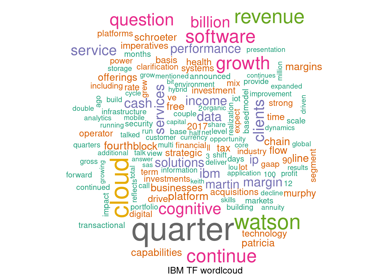
##    user  system elapsed
##   0.521   0.009   0.436
And now, test driving the IDF one…
system.time({ build_wordcloud(dtm_ibm_idf, plot.title="IBM IDF wordlcoud", min.freq=2) }) # 0.09 secs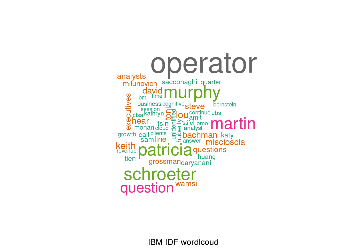
##    user  system elapsed
##   0.321   0.007   0.214
1.5.6 Func 4: Simple Bar.charts of top tokens
Self-explanatory. And simple. But just for completeness sake, making a func out of it.
 plot.barchart <- function(dtm, num_tokens=15, fill_color="Blue")
 {
 a0 = apply(dtm, 2, sum)
 a1 = order(a0, decreasing = TRUE)
 tsum = a0[a1]

 # plot barchart for top tokens
 test = data.frame(term = names(tsum)[1:num_tokens], freq=round(tsum[1:num_tokens],0)); test

 # windows()  # New plot window
 require(ggplot2)
 p = ggplot(test, aes(x = term, y = freq)) +
       geom_bar(stat = "identity", fill = fill_color) +
       geom_text(aes(label = freq), vjust= -0.20) +
       theme(axis.text.x = element_text(angle = 90, hjust = 1))

 plot(p) }  # func ends

 # testing above func
 system.time({ plot.barchart(dtm_ibm_tf) })    # 0.1 secs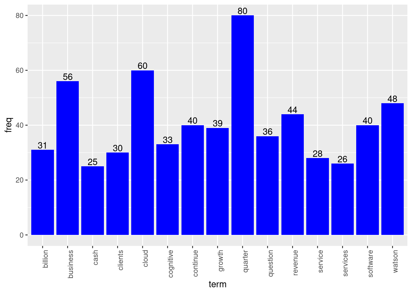
##    user  system elapsed
##   0.089   0.000   0.087
# system.time({ plot.barchart(dtm_ibm_idf, num_tokens=12, fill_color="Red") }) # 0.11 secs1.5.7 Func 5: Co-occurrence graphs (COGs)
COGs as the ame suggests connects those tokens together that most co-occur within documents, using a network graph wherein the nodes are tokens of interest.
This is admittedly a slightly long-winded func. Also introduces network visualization concepts. If you’re unfamiliar with this, pls execute the func’s content line-by-line to see what each line does.
 distill.cog = function(dtm, # input dtm
                       title="COG", # title for the graph
                       central.nodes=4,    # no. of central nodes
                       max.connexns = 5){  # max no. of connections

 # first convert dtm to an adjacency matrix
 dtm1 = as.matrix(dtm)   # need it as a regular matrix for matrix ops like %*% to apply
 adj.mat = t(dtm1) %*% dtm1    # making a square symmatric term-term matrix
 diag(adj.mat) = 0     # no self-references. So diag is 0.
 a0 = order(apply(adj.mat, 2, sum), decreasing = T)   # order cols by descending colSum
 mat1 = as.matrix(adj.mat[a0[1:50], a0[1:50]])

  # now invoke network plotting lib igraph
  library(igraph)

  a = colSums(mat1) # collect colsums into a vector obj a
  b = order(-a)     # nice syntax for ordering vector in decr order

  mat2 = mat1[b, b]     # order both rows and columns along vector b
  diag(mat2) =  0

  ## +++ go row by row and find top k adjacencies +++ ##

  wc = NULL

  for (i1 in 1:central.nodes){
    thresh1 = mat2[i1,][order(-mat2[i1, ])[max.connexns]]
    mat2[i1, mat2[i1,] < thresh1] = 0   # neat. didn't need 2 use () in the subset here.
    mat2[i1, mat2[i1,] > 0 ] = 1
    word = names(mat2[i1, mat2[i1,] > 0])
    mat2[(i1+1):nrow(mat2), match(word,colnames(mat2))] = 0
    wc = c(wc, word)
  } # i1 loop ends


  mat3 = mat2[match(wc, colnames(mat2)), match(wc, colnames(mat2))]
  ord = colnames(mat2)[which(!is.na(match(colnames(mat2), colnames(mat3))))]  # removed any NAs from the list
  mat4 = mat3[match(ord, colnames(mat3)), match(ord, colnames(mat3))]

  # building and plotting a network object
  graph <- graph.adjacency(mat4, mode = "undirected", weighted=T)    # Create Network object
  graph = simplify(graph)
  V(graph)$color[1:central.nodes] = "green"
  V(graph)$color[(central.nodes+1):length(V(graph))] = "pink"

  graph = delete.vertices(graph, V(graph)[ degree(graph) == 0 ]) # delete singletons?

  plot(graph,
       layout = layout.kamada.kawai,
       main = title)

  } # distill.cog func ends

 # testing COG on ibm data
 system.time({ distill.cog(dtm_ibm_tf, "COG for IBM TF") })    # 0.27 secs
## Warning in vattrs[[name]][index] <- value: number of items to replace is not a
## multiple of replacement length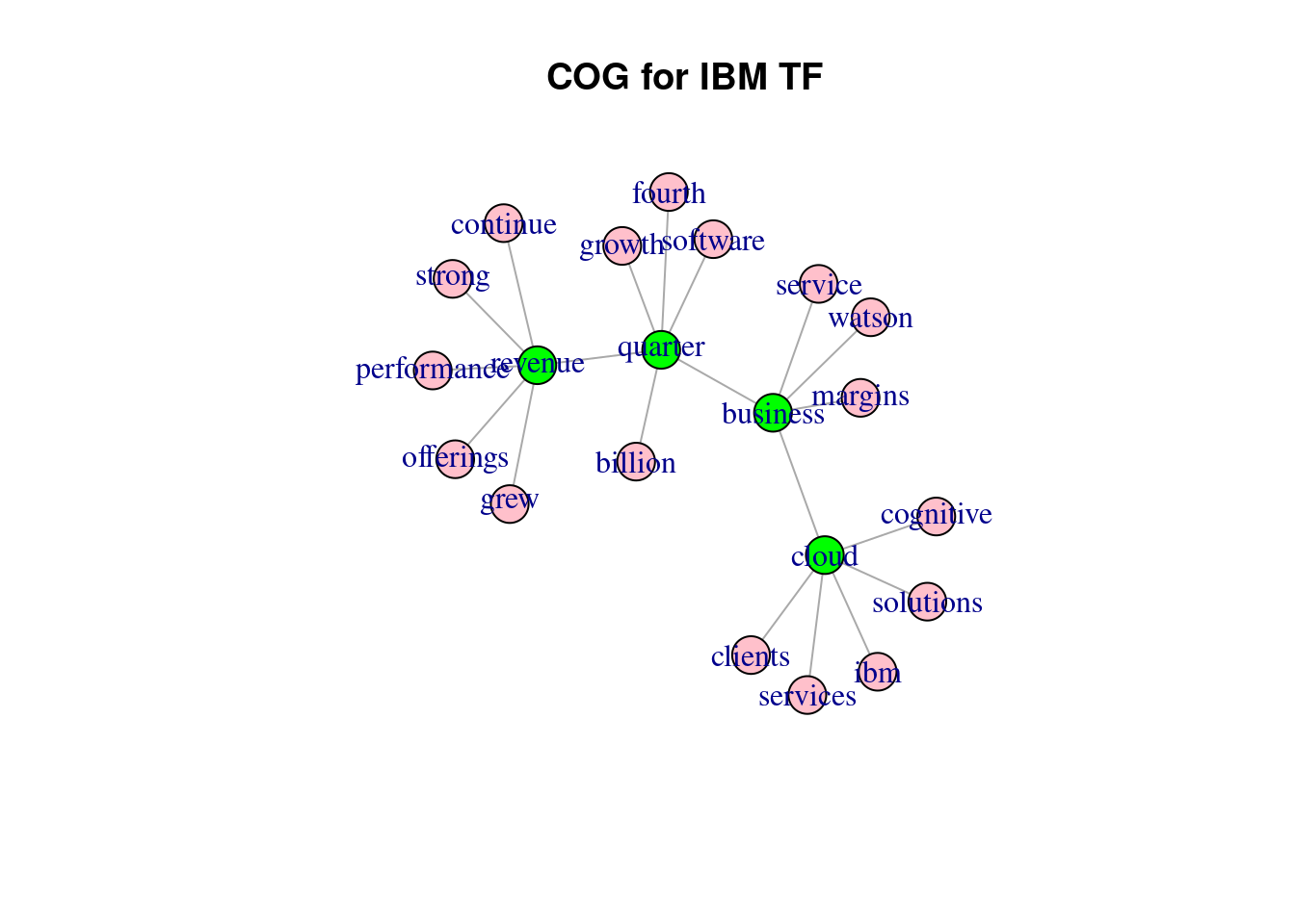
##    user  system elapsed
##   0.412   0.012   0.418
# system.time({ distill.cog(dtm_ibm_idf, "COG for IBM IDF", 5, 5) }) # 0.57 secs1.5.8 Func 6 - wordcloud + COG combo
Both the 2 major display aids we saw thus far - cog and wordcloud - have their pros and cons. Can we somehow combine them and get the best of both worlds, so to say? Read on.
 build_cog_ggraph <- function(corpus,   # text colmn only
                             max_edges = 150,
                             drop.stop_words=TRUE,
                             new.stopwords=NULL){

  # invoke libraries
  library(tidyverse)
  library(tidytext)
  library(widyr)
  library(ggraph)

  # build df from corpus
  corpus_df = data.frame(docID = seq(1:length(corpus)), text = corpus, stringsAsFactors=FALSE)

  # eval stopwords condn
  if (drop.stop_words == TRUE) {stop.words = unique(c(stop_words$word, new.stopwords)) %>%
    as_tibble() %>% rename(word=value)} else {stop.words = stop_words[2,]}

  # build word-pairs
  tokens <- corpus_df %>%

    # tokenize, drop stop_words etc
    unnest_tokens(word, text) %>% anti_join(stop.words)

    # pairwise_count() counts #token-pairs co-occuring in docs
  word_pairs = tokens %>% pairwise_count(word, docID, sort = TRUE, upper = FALSE)# %>% # head()

  word_counts = tokens %>% count( word,sort = T) %>% dplyr::rename( wordfr = n)

  word_pairs = word_pairs %>% left_join(word_counts, by = c("item1" = "word"))

  row_thresh = min(nrow(word_pairs), max_edges)

  # now plot
  set.seed(1234)
  # windows()
  plot_d <- word_pairs %>%
    filter(n >= 3) %>%
    top_n(row_thresh) %>%   igraph::graph_from_data_frame()

  dfwordcloud = data_frame(vertices = names(V(plot_d))) %>% left_join(word_counts, by = c("vertices"= "word"))

  plot_obj = plot_d %>%   # graph object built!

    ggraph(layout = "fr") +
    geom_edge_link(aes(edge_alpha = n, edge_width = n), edge_colour = "cyan4")  +
    # geom_node_point(size = 5) +
    geom_node_point(size = log(dfwordcloud$wordfr)) +
    geom_node_text(aes(label = name), repel = TRUE,
                   point.padding = unit(0.2, "lines"),
                   size = 1 + log(dfwordcloud$wordfr)) +
    theme_void()

  return(plot_obj)    # must return func output

 }  # func ends

 # quick example for above using amazon nokia corpus
 nokia = readLines('https://github.com/sudhir-voleti/sample-data-sets/raw/master/text%20analysis%20data/amazon%20nokia%20lumia%20reviews.txt')
 system.time({ b0=build_cog_ggraph(nokia) })    # 0.36 secs
## Joining, by = "word"## Warning: `distinct_()` was deprecated in dplyr 0.7.0.
## Please use `distinct()` instead.
## See vignette('programming') for more help
## This warning is displayed once every 8 hours.
## Call `lifecycle::last_lifecycle_warnings()` to see where this warning was generated.## Selecting by wordfr## Warning: `data_frame()` was deprecated in tibble 1.1.0.
## Please use `tibble()` instead.
## This warning is displayed once every 8 hours.
## Call `lifecycle::last_lifecycle_warnings()` to see where this warning was generated.## user system elapsed
## 0.279 0.003 0.281 b0## Warning: ggrepel: 2 unlabeled data points (too many overlaps). Consider
## increasing max.overlaps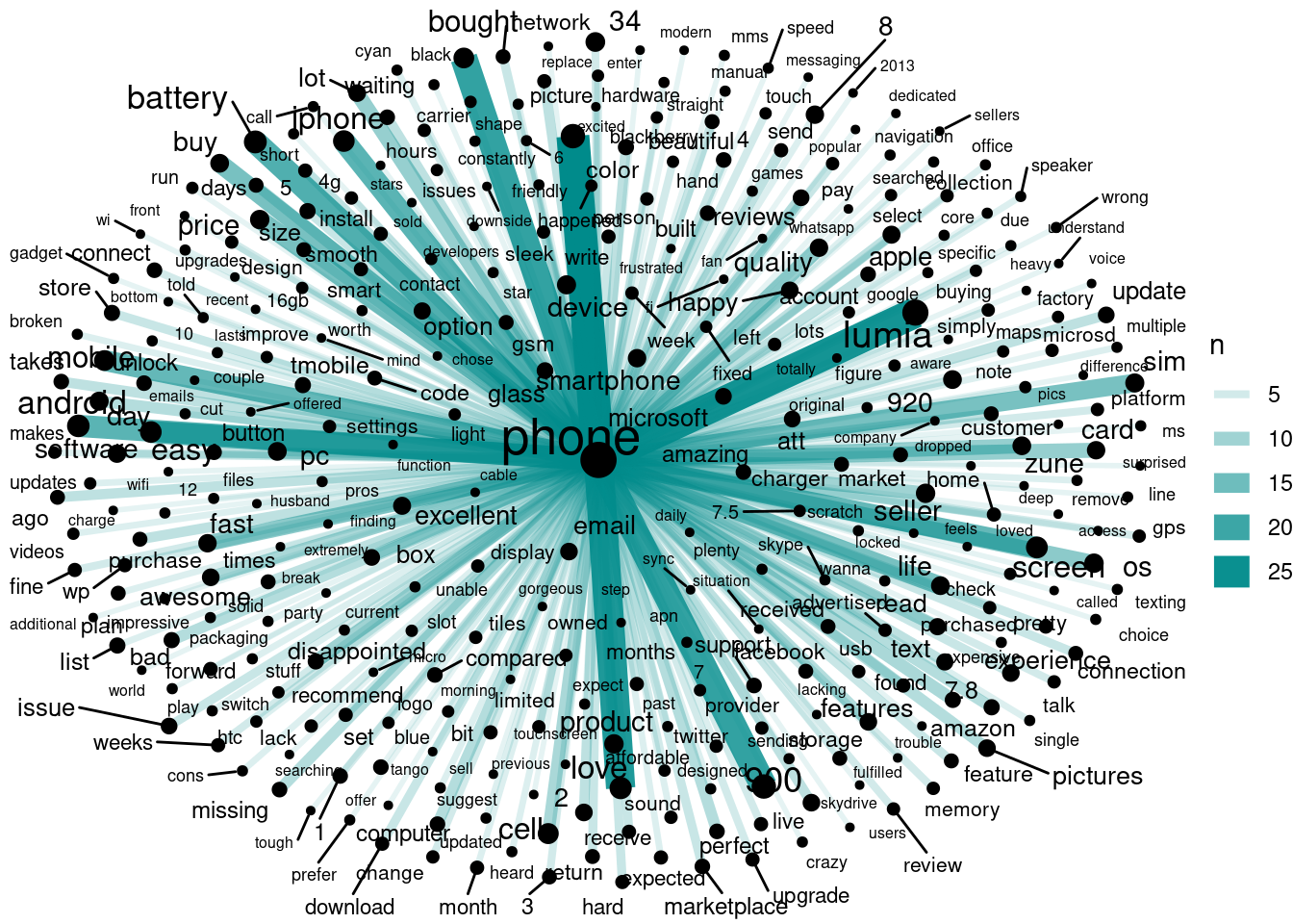
Clearly, the most frequently occurring token above has taken epi-central node status. What if we dropped it? What new patterns might emerge? Points to ponder…
1.6 Tidytext funcs based exercise
Creatively apply our basic text-an funcs to the file ‘ice-cream data.txt’ available at this link:
https://raw.githubusercontent.com/sudhir-voleti/sample-data-sets/master/Ice-cream-dataset.txt
Now answer these Qs:
- What was the size of the DTM finally built?
- Which stand-alone (or single) flavours seem to be the most popular?
- Which flavour combinations (2 or more) seem to be popular?
- What display aids did you use to answer the above questions?
Well, that’s it for now. I’m sure I have run out of time. If so, will pickup in the next session from where we leave off.
Sudhir
1.7 Homebrewing DTMs and n-grams
1.7.1 Introduction to this markdown
We saw how to home-brew a simple tokenizer from first principles. P.S. Coders sometimes refer to cooking up one’s own functions as home-brewing.
After tokenization, certain other steps in text-an follow. Such as, building Document Term Matrices (DTMs), n-grams of interest, etc.
Now R has several libraries that perform these tasks. But before we go there, the aim is to once, quickly, home-brew these critical data structures, then it helps build and extend our understanding, as well as confidence.
1.7.2 Invoking the Home-brewed tokenizer
Let’s quickly read-in the tokenizers we built. Then we’ll extend / build on top of them and arrive at home-brewed DTMs and n-grams.
# first things first
rm(list = ls())   # clears workspace
library(stringr)
Now the two funcs themselves - Tokenize_String() and Tokenize_Text_Block() - see code below, borrowed from the last RMD.
P.S. Note func naming convention here: Am using capitalized phrases for func names, unlike previously. Feel free to follow any naming convention you want to, as long as it logical and consistent.
# Re-read the two 'home-brewed' tokenizer functions we'd built.
Tokenize_String <- function(string){

  temp <- tolower(string)   # Lowercase

  temp <- stringr::str_replace_all(temp,"[^a-zA-Z\\s]", " ") # replace non-alphabets with \s

  temp <- stringr::str_replace_all(temp,"[\\s]+", " ") # collapse >1 spaces into 1 space

  temp <- stringr::str_split(temp, " ")[[1]]

  indexes <- which(temp == "")
  if(length(indexes) > 0){ temp <- temp[-indexes]  }
  return(temp)

} # Tokenize_String func ends
We defined a unit func above, for single strings.
Next, we’ll wrap the unit func into a larger ‘wrapper’ func defined over collections of strings. Behold.
# This below is the Tokenizer for text blocks
Tokenize_Text_Block <- function(text){

      # Check to see if there is any text at all with another conditional
      if(length(text) == 0){ cat("There was no text in this document! \n"); stop }

      # Get rid of blank lines
      indexes <- which(text == "")
      if(length(indexes) > 0){ text <- text[-indexes]   }

      # Loop through the lines in the text and use the append() function to
      clean_text <- Tokenize_String(text[1])
      if (length(text)>1){

        for(i in 2:length(text)){
        # add them to a vector
        clean_text <- append(clean_text, Tokenize_String(text[i])) }   # i loop ends

            } # if condn ends

      # Calc number of tokens and unique tokens. Return them in a named list object.
      num_tok <- length(clean_text)
      num_uniq <- length(unique(clean_text))

      to_return <- list(num_tokens = num_tok,   # output is list with 3 elements
                        unique_tokens = num_uniq,
                        text = clean_text)

    return(to_return)
} # Tokenize_Text_Block func ends
As an example, we consider a small text corpus. Specifically the first 2 paragraphs from the Wikipedia page on ISB.
# Reading in an ISB example (first two paras from Wiki)
text.para1 <- "Indian School of Business (ISB), is one of the prestigious business schools in India and is rated amongst the best in the world .The institute has various management programs with the PGP as its flagship course .Admission to the coveted management program is rigorous and has also the distinction of having one of the most stringent selectivity ratio internationally . The student cohort has a diverse mix with students coming in from top Indian and International Universities like the IITs , BITS Pilani, NITs , SRCC , ISI etc. There are students who are doctors , people from defence establishments ,sportsman and who have excelled in various other professions .ISB has integrated campuses at Mohali, Punjab and Hyderabad, Telangana, and is a non profit organization.[2] The school was founded by two senior executives of McKinsey & Company with the backing of government and is governed by a board comprising both Indian and non-Indian businessmen."
text.para1
## [1] "Indian School of Business (ISB), is one of the prestigious business schools in India and is rated amongst the best in the world .The institute has various management programs with the PGP as its flagship course .Admission to the coveted management program is rigorous and has also the distinction of having one of the most stringent selectivity ratio internationally . The student cohort has a diverse mix with students coming in from top Indian and International Universities like the IITs , BITS Pilani, NITs , SRCC , ISI etc. There are students who are doctors , people from defence establishments ,sportsman and who have excelled in various other professions .ISB has integrated campuses at Mohali, Punjab and Hyderabad, Telangana, and is a non profit organization.[2] The school was founded by two senior executives of McKinsey & Company with the backing of government and is governed by a board comprising both Indian and non-Indian businessmen."This below is Para 2.
text.para2 <- "ISB has been ranked 27th in the world in the 2017 Financial Times Global MBA Rankings.[3] It is the first business school in Indian subcontinent to be accredited by the Association to Advance Collegiate Schools of Business.[4] In 2008, it became the youngest institution to find a place in global MBA rankings when it was ranked 20.[5] Indian School of Business accepts both GMAT and GRE scores for the admission process."
text.para2
## [1] "ISB has been ranked 27th in the world in the 2017 Financial Times Global MBA Rankings.[3] It is the first business school in Indian subcontinent to be accredited by the Association to Advance Collegiate Schools of Business.[4] In 2008, it became the youngest institution to find a place in global MBA rankings when it was ranked 20.[5] Indian School of Business accepts both GMAT and GRE scores for the admission process."Now, we invoke the funcs above and tokenize these paragraphs.
# tokenize these paragraphs
out.para1 = Tokenize_Text_Block(text.para1)
out.para2 = Tokenize_Text_Block(text.para2)
str(out.para1)   # check the structure or str() of the output
## List of 3
## $ num_tokens : int 149
## $ unique_tokens: int 97
## $ text : chr [1:149] "indian" "school" "of" "business" ...1.8 Building DTM from first principles
We know that text corpora are organized along broad units called ‘documents’ which we can define. These could be individual reviews, tweets, paragraphs in an unbroken text article etc.
A DTM or *document-term-matrix** is a matrix with one row per document and one column per unique token. Each cell [i, j] in the DTM carries the number of occurrences of token j in document i.
From the above, we know how to tokenize text into word-tokens. Now let’s home-brew a DTM on that basis.
# Merge the two token sets
merged.token.sets = unique(c(out.para1$text, out.para2$text))
length(merged.token.sets)
## [1] 125Next we pre-define the DTM object. Pay thought to why we should do this.
In R, it’s better to pre-define objects’ sizes so that R can allocate memory at the beginning in a static, stable way.
Functions such as rbind() or cbind() dynamically append more rows or columns (respectively) to data objects requiring dynamic memory allocation, which R isn’t great at.
The DTM will have as many rows as there are docs (2 in our ISB example) and as many columns as there are unique tokens. So…
# define the dtm object to populate
dtm.fp = matrix(0, nrow = 2, ncol = length(merged.token.sets))
  row.names(dtm.fp) = seq(1:2)
  colnames(dtm.fp) = merged.token.sets
dim(dtm.fp)
## [1] 2 125# define rows in a list
docs.list = list(out.para1$text, out.para2$text)Now its time to populate the DTM.
There’re many ways to achieve this. I’m using a simple approach - for loops - that’s intuitive but not efficient. See code below.
# populate the dtm
for (i1 in 1:length(merged.token.sets)){    # looping over tokens

  for (i2 in 1:2){    # loop over documents

      dtm.fp[i2, i1] = length(grep(merged.token.sets[i1], docs.list[[i2]]))

}} # both i1, i2 loops end

dtm.fp[, 1:15]    # view first 15 cols of the DTM
## indian school of business isb is one the prestigious schools in india and
## 1 4 3 8 3 2 12 2 14 1 1 23 5 8
## 2 2 3 2 3 1 3 0 6 0 1 16 2 1
## rated amongst
## 1 2 1
## 2 0 0The interpretation of the resulting table is straightforward. The DTM above says that the tokens ‘indian’ and ‘school’ occurred 4 and 3 times respectively in document 1, and {2, 3} times respectively in document 2. And so on.
DTMs are so fundamental to text-An that almost every text-an library in R (or Py, for that matter) will have in-built tokenizer plus DTM builder functions.
And now that we have seen how to home-brew DTMs, we can: * (i) open up these functions to see their innards, and * (ii) change things as required by particular problem contexts.
1.8.1 Building a simple n-gram tokenizer
Next we home-brew n-grams. A single word, say “cream”, is a unigram.
But two (or more) words such as “ice” and “cream” that tend to occur together form a phrase (or part thereof) and can be identified as unique tokens in their own right.
Thus, “ice cream” is a bi-gram whereas “ice cream cone” would be a tri-gram.
Mind you, n-grams aren’t just any 2 or 3 words that occurred somewhere once together but are repeated (partial) phrases that occur multiple times through the corpus.
# build matrix to hold (n-1) bigrams
n = length(out.para1$text); n
## [1] 149bigram.mat = matrix(0, nrow = (n-1), ncol = 2)A sentence with 5 words - say, “My name is Amitabh Bachchan” - has 4 sets of consecutive word-pairs in it, namely “My name”, “name is”, “is Amitabh”, and “Amitabh Bachchan”.
More generally, any text with n tokens can have at most (n-1) bigrams in it. Likewise, (n-2) trigrams and so on.
# loop over all tokens now
for (i1 in 1:(n-1)){

  bigram.mat[i1, 1] = out.para1$text[i1]
  bigram.mat[i1, 2] = out.para1$text[i1+1]
  }

head(bigram.mat)
## [,1] [,2]
## [1,] "indian" "school"
## [2,] "school" "of"
## [3,] "of" "business"
## [4,] "business" "isb"
## [5,] "isb" "is"
## [6,] "is" "one"And now it’s easy to stitch up the two unigram components into a bigram using paste(), thus:
stitched = paste(bigram.mat[,1], bigram.mat[,2], sep=".")
bigram_df = data.frame(unigram1 = bigram.mat[,1], unigram2 = bigram.mat[,2], bigram = stitched)
head(bigram_df)
## unigram1 unigram2 bigram
## 1 indian school indian.school
## 2 school of school.of
## 3 of business of.business
## 4 business isb business.isb
## 5 isb is isb.is
## 6 is one is.oneWhile we see many word-pairs, how many are true bi-grams? How about we run a de-duplication on the matrix’s rows and find out?
a0 = unique.matrix(bigram.mat); dim(a0) # how many bigrams occurred multiple times.## [1] 142 2And the same applies to trigrams as well. See code below.
# the same for trigrams is just as easy
trigram.mat = matrix(0, nrow = (n-2), ncol = 3)

for (i1 in 1:(n-2)){
  trigram.mat[i1, 1] = out.para1$text[i1]
  trigram.mat[i1, 2] = out.para1$text[i1+1]
  trigram.mat[i1, 3] = out.para1$text[i1+2]
}

head(trigram.mat)
## [,1] [,2] [,3]
## [1,] "indian" "school" "of"
## [2,] "school" "of" "business"
## [3,] "of" "business" "isb"
## [4,] "business" "isb" "is"
## [5,] "isb" "is" "one"
## [6,] "is" "one" "of"With that, I’ll stop home-brewing here. We’ll next go to standard R libraries and directly use their DTM and n-gram functions here on.
Sudhir