4 Data Processing

4.1 Gene body coverage

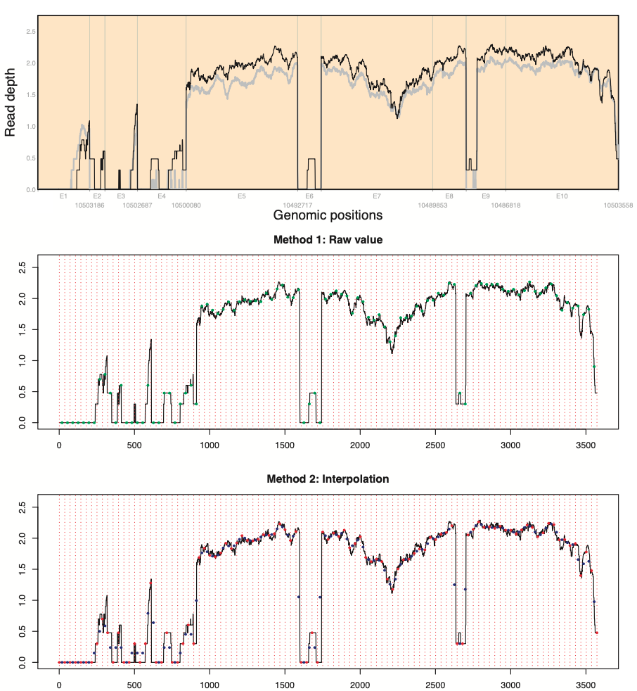
The union transcript is used to extract only exon pileup. To keep only exon location, we first build coverage pileup from raw pileup (part_intron) to pileupData (only_exon). By comparing the dimension of pileup using get_pileupExon function or saved *_pileup_part_intron.RData, we can notice the adjustment for the effect of gene length is required. norm_pileup.* functions have two options to select read depth at the region: raw value and interpolation. After evenly dividing genomic positions by the number of regions (red vertical broken lines), suppose that both sides and center of regions are x-values of odd and even points, respectively. While the first method finds read depth at even points (green points), and the second one finds geometric mean (blue points) using read depth at odd points (red points). We recommend using the gene length normalization methods for gene length is at least 2\(\times\)the number of regions+1 to secure minimum read depth selection across genes.

Before the coverage normalization, identification and filter low-expression genes need by the filter_lowExpGenes function to reduce sampling noise. Only 961 out of 1,000 genes are used for gene body coverage if you consider genes with smaller percentages of TPM < 5 than 50%. Genes are separated into two groups to compare base coverage patterns in short and long genes. 0~5 kb and 5+ kb cover 96 and 865 genes, respectively.

pileupPath <- paste0("../pileup/", genelist, "_pileup_part_intron.RData")

# Filtered genes
genelist2 <- filter_lowExpGenes(genelist, TPM, thru=5, pct=50)
pileupPath2 <- paste0("../pileup/", genelist2, "_pileup_part_intron.RData")

geneInfo2 <- geneInfo[match(genelist2, geneInfo$geneSymbol), ] %>%
  mutate(merged_kb=merged/1000,
         Len=factor(case_when(
           merged_kb>=0 & merged_kb<5 ~ "0~5 kb",
           merged_kb>=5 ~ "5+ kb",
           is.na(merged_kb) ~ NA)),
         LenSorted=forcats::fct_relevel(Len, "0~5 kb", "5+ kb")
  )

table(geneInfo2$LenSorted)

## 
## 0~5 kb  5+ kb 
##     96    865

genelist2Len0 <- geneInfo2[geneInfo2$LenSorted=="0~5 kb", c("geneSymbol")]
pileupPath2Len0 <- paste0("../pileup/", genelist2Len0, "_pileup_part_intron.RData")

genelist2Len5 <- geneInfo2[geneInfo2$LenSorted=="5+ kb", c("geneSymbol")]
pileupPath2Len5 <- paste0("../pileup/", genelist2Len5, "_pileup_part_intron.RData")

In the plot_GBC function, evenly spaced regions are defined as gene body percentile where the number of regions is 100. Unstable patterns in base coverage especially in short genes are still detected even after filtering low-expression genes.

GBC0 = plot_GBC(pileupPath2Len0, geneNames=genelist2Len0, rnum=100, method=1, scale=TRUE, stat=2, plot=TRUE, sampleInfo)
GBC5 = plot_GBC(pileupPath2Len5, geneNames=genelist2Len5, rnum=100, method=1, scale=TRUE, stat=2, plot=TRUE, sampleInfo)

p0 <- GBC0$plot +
  coord_cartesian(ylim=c(0, 0.017)) +
  ggtitle("0~5 kb")
p5 <- GBC5$plot +
  coord_cartesian(ylim=c(0, 0.017)) +
  ggtitle("5+ kb")

ggpubr::ggarrange(p0, p5, common.legend=TRUE, legend="bottom", nrow=1)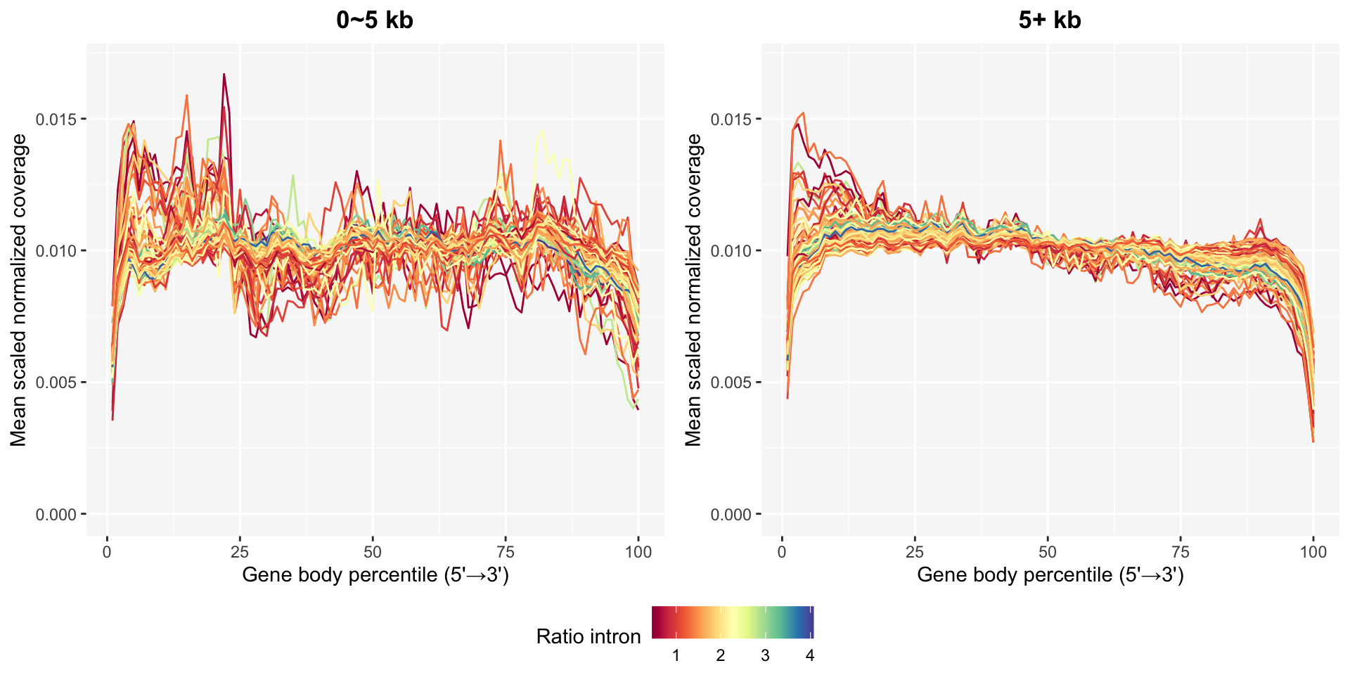

4.2 CVs per level

Metrics from scaled normalized transcript coverage for samples can be calculated by the get_metrics function. The sample level robustCV can be employed to compare trends with other sample properties and window CV matrix.

met = get_metrics(pileupPath, geneNames=genelist, rnum=100, method=1, scale=TRUE, margin=1)
head(round(met, 4))

##                     mean     sd     CV median    mad robustCV
## S000004-37958-003 0.0103 0.0033 0.3156 0.0105 0.0031   0.2957
## S000004-38071-002 0.0104 0.0032 0.3139 0.0106 0.0030   0.2886
## S000004-38094-003 0.0103 0.0033 0.3187 0.0105 0.0032   0.2998
## S000004-38120-002 0.0105 0.0035 0.3353 0.0107 0.0034   0.3165
## S000004-38134-002 0.0105 0.0035 0.3364 0.0106 0.0033   0.3130
## S000004-38138-003 0.0107 0.0039 0.3686 0.0108 0.0039   0.3580