Working title: Voters want mayors with driver’s licence, but do elected representatives know it?

Abstract

Candidate choice studies around the world refute the notion that sociodemographic groups are underrepresented in politics because they are low in demand among voters. Are party gate-keepers to blame? We contribute to the study of demand-side effects of political candidates by investigating whether underrepresented candidates face demand-side hurdles within political parties. Specifically, we field a candidate conjoint experiment simultaneously to voters and a panel of politicians, asking the voters which candidate they want for mayor in their municipality and asking the politicians which candidate they believe the voters want for mayor. The candidates’ attributes vary along dimensions of age, gender, religious background, education level, and political experience.

Introduction

Democratic systems rely on electing willing citizens to make decisions on behalf of everyone. Although the principle of equal participation informs these processes, some social groups remain underrepresented, which may raise concerns about fair political influence (Butler 2014; Carnes 2012; Carnes and Lupu 2023; Mansbridge 1999; Mathisen 2024). At the core of these worries lies the assumption that descriptive characteristics—such as gender, education, religion, or ethnicity—can shape political attitudes and behaviors in ways that matter for representation. Many studies indicate that voters interpret candidates’ demographic or social backgrounds as signals for policy stances (Brady and Sniderman 1985; Arnesen, Duell, and Johannesson 2019).

From the demand-side perspective, attention centers on the voters’ preferences regarding who should represent them. One method for studying these preferences is the candidate conjoint experiment (Hainmueller, Hopkins, and Yamamoto 2014; Kirkland and Coppock 2018). In such experiments, participants in a survey see profiles of two hypothetical candidates randomly assigned attributes—for example, religion, ethnicity, age, gender, and education level—and are asked to choose which candidate they prefer. Because the attributes vary randomly, researchers can statistically isolate the effect of each characteristic on voter choice.

The rapid expansion of candidate choice studies over the last decade reveals patterns that occasionally run counter to real-world representation. For instance, while many legislatures are male-dominated, a growing body of conjoint research suggests that voters tend to favor female over male candidates, on average (Schwarz and Coppock 2022). Meta-studies show that candidates of older age are over-represented among political representatives, even though voters on average tend to prefer middle-aged candidates (Eshima and Smith 2022; McClean and Ono 2024). Voters do not penalize ethnic minorities in candidate choice experiments, but they are often underrepresented in legislative bodies (Oosten, Mügge, and Pas 2024). What causes this discrepancy?

For one, what the voters state in surveys may be different from how they behave in real elections. However, previous studies indicate that what respondents state in conjoint experiments is closely aligned with their real-world behavior (Hainmueller, Hangartner, and Yamamoto 2015). Then there is the issue of supply-side dynamics, which may work in disfavor of citizens of certain backgrounds. They may—on average and for various reasons—have lower motivation, smaller networks, and fewer resources needed to enter and become successful in politics (Verba, Schlozman, and Brady 1995).

The question is large in scope and has several explanations beyond the scope of a single study. In this study, we contribute to the literature by focusing on one specific, understudied demand-side explanation: how elected representatives perceive the electability of mayor candidates based on the candidates’ social background. In Norway and many other political systems, elected representatives serve as gatekeepers, having the final say in who to choose as mayor candidates for their party. One of the main considerations they make concerns electability:

which of the potential candidates is more popular among the electorate? While every context is unique, it is quite plausible that party members pay attention to the candidates’ background as part of their assessment in selecting their preferred candidate. They should, and we expect them to do so, given the clear findings across the world that voters differentiate between candidates on this basis. But are their assessments accurate?

To investigate this, we survey elected representatives in Norway, asking them in a candidate conjoint design to assess what types of mayoral candidates they believe the voters demand. We also field and compare their opinions with the results of a similar conjoint design of a representative sample of citizens in Norway. We thus field the experiment in parallel in representative online panels of citizens and elected representatives in Norway. The design is identical across the two samples, with the exception that whereas the voters are asked which candidate they would pick out of two profiles, the elected representatives are asked which candidate they think the voters would pick.

We estimate the results using marginal means of the two samples, and the differences marginal means between the two samples (Leeper, Hobolt, and Tilley 2018). Below we outline the code for our analysis plan.

R Script for Analysis Plan

R Session Info and Load libraries

Code

# Set Global Options

knitr::opts_chunk$set(
  echo = TRUE,      # Show code in output
  warning = FALSE,  # Hide warnings
  message = FALSE,  # Hide messages
  fig.width = 7,    # Set figure width
  fig.height = 5,   # Set figure height
  fig.align = "center" # Align figures in the center
)

sessionInfo()

R version 4.3.1 (2023-06-16 ucrt)
Platform: x86_64-w64-mingw32/x64 (64-bit)
Running under: Windows 11 x64 (build 22631)

Matrix products: default


locale:
[1] LC_COLLATE=English_United States.utf8 
[2] LC_CTYPE=English_United States.utf8   
[3] LC_MONETARY=English_United States.utf8
[4] LC_NUMERIC=C                          
[5] LC_TIME=English_United States.utf8    

time zone: Europe/Oslo
tzcode source: internal

attached base packages:
[1] grid      stats     graphics  grDevices utils     datasets  methods  
[8] base     

other attached packages:
 [1] readxl_1.4.3           patchwork_1.3.0        ggforce_0.4.2         
 [4] broom.helpers_1.17.0   marginaleffects_0.24.0 scales_1.3.0          
 [7] survey_4.4-2           survival_3.8-3         Matrix_1.5-4.1        
[10] cregg_0.4.0            broom_1.0.7            haven_2.5.4           
[13] lubridate_1.9.4        forcats_1.0.0          stringr_1.5.1         
[16] dplyr_1.1.4            purrr_1.0.2            readr_2.1.5           
[19] tidyr_1.3.1            tibble_3.2.1           ggplot2_3.5.1         
[22] tidyverse_2.0.0        kableExtra_1.4.0      

loaded via a namespace (and not attached):
 [1] gtable_0.3.6      xfun_0.49         htmlwidgets_1.6.4 lattice_0.22-6   
 [5] tzdb_0.4.0        vctrs_0.6.5       tools_4.3.1       generics_0.1.3   
 [9] sandwich_3.1-1    fansi_1.0.6       pkgconfig_2.0.3   data.table_1.16.4
[13] lifecycle_1.0.4   farver_2.1.2      compiler_4.3.1    munsell_0.5.1    
[17] ggstance_0.3.7    mitools_2.4       htmltools_0.5.8.1 yaml_2.3.8       
[21] pillar_1.9.0      MASS_7.3-60       tidyselect_1.2.1  digest_0.6.34    
[25] stringi_1.8.4     splines_4.3.1     polyclip_1.10-7   fastmap_1.2.0    
[29] colorspace_2.1-0  cli_3.6.2         magrittr_2.0.3    utf8_1.2.4       
[33] withr_3.0.2       backports_1.5.0   timechange_0.3.0  rmarkdown_2.29   
[37] cellranger_1.1.0  zoo_1.8-12        hms_1.1.3         evaluate_1.0.1   
[41] knitr_1.49        lmtest_0.9-40     viridisLite_0.4.2 rlang_1.1.3      
[45] Rcpp_1.0.13-1     glue_1.7.0        DBI_1.2.3         tweenr_2.0.3     
[49] xml2_1.3.6        svglite_2.1.3     rstudioapi_0.17.1 jsonlite_1.8.9   
[53] R6_2.5.1          systemfonts_1.1.0

Code

setwd("C:/Users/svein/OneDrive - NORCE/Prosjekter/Immigrant inclusion/Valgbarhet")

library(kableExtra)       # tidy tables
library(tidyverse)        # ggplot, dplyr, and friends
library(ggplot2)
library(haven)            # Read Stata files
library(broom)            # Convert model objects to tidy data frames
library(cregg)            # Automatically calculate frequentist conjoint AMCEs and MMs
library(survey)           # Panel-ish regression models
library(scales)           # Nicer labeling functions
library(marginaleffects)  # Calculate marginal effects
library(broom.helpers)    # Add empty reference categories to tidy model data frames
library(ggforce)          # For facet_col()
library(patchwork)        # Combine ggplot plots
library(readxl)           # Read Excel files

Set Up Theme and Functions

Code

# Inspired by Andrew Heiss https://www.andrewheiss.com/blog/2023/07/25/conjoint-bayesian-frequentist-guide/#marginal-means

library(ggplot2)
library(scales)  
library(tidyverse)

── Attaching core tidyverse packages ──────────────────────── tidyverse 2.0.0 ──
✔ dplyr     1.1.4     ✔ readr     2.1.5
✔ forcats   1.0.0     ✔ stringr   1.5.1
✔ lubridate 1.9.4     ✔ tibble    3.2.1
✔ purrr     1.0.2     ✔ tidyr     1.3.1
── Conflicts ────────────────────────────────────────── tidyverse_conflicts() ──
✖ readr::col_factor() masks scales::col_factor()
✖ purrr::discard()    masks scales::discard()
✖ dplyr::filter()     masks stats::filter()
✖ dplyr::lag()        masks stats::lag()
ℹ Use the conflicted package (<http://conflicted.r-lib.org/>) to force all conflicts to become errors

Code

# Define theme function 
theme_nice <- function() {
  theme_minimal(base_family = "Jost") +
    theme(panel.grid.minor = element_blank(),
          plot.title = element_text(family = "Jost", face = "bold"),
          axis.title = element_text(family = "Jost Medium"),
          axis.title.x = element_text(hjust = 0),
          axis.title.y = element_text(hjust = 1),
          strip.text = element_text(family = "Jost", face = "bold",
                                    size = rel(0.75), hjust = 0),
          strip.background = element_rect(fill = "grey90", color = NA))
}

# Set the default theme *after* defining it
theme_set(theme_nice())

# Update default font settings
update_geom_defaults("text", list(family = "Jost", fontface = "plain"))
update_geom_defaults("label", list(family = "Jost", fontface = "plain"))


# Colors for heterogeneous effects
parties <- c("#1696d2", "#db2b27")


# Functions for formatting things as percentage points
label_pp <- label_number(accuracy = 1, scale = 100, 
                         suffix = " pp.", style_negative = "minus")

label_amce <- label_number(accuracy = 0.1, scale = 100, suffix = " pp.", 
                           style_negative = "minus", style_positive = "plus")

Load and Generate Data

Code

# NCP data
# df_ncp <- read_sav("Norsk medborgerpanel - runde 31 - v-100-O.sav") #for when we get all data
df_ncp <- read_excel("Data/r31_poelex_sample_publicid_i2e_2024_12_09.xlsx")

# data <- data %>% 
#   select(responseid, starts_with("r31_poelex"), r31_pcpar_raw) %>%
#   rename(rsp_vote = r31_pcpar_raw) # for when we get all data

head(df_ncp)

# A tibble: 6 × 17
  responseid    r31_poelex_religion1 r31_poelex_religion2 r31_poelex_innvandri…¹
  <chr>                        <dbl>                <dbl>                  <dbl>
1 425243584468…                    3                    2                      2
2 425243582651…                    3                    2                      1
3 425243592616…                    2                    1                      1
4 425243592186…                    2                    3                      2
5 425243592681…                    1                    1                      2
6 425243588423…                    3                    2                      1
# ℹ abbreviated name: ¹​r31_poelex_innvandring1
# ℹ 13 more variables: r31_poelex_innvandring2 <dbl>, r31_poelex_alder1 <dbl>,
#   r31_poelex_alder2 <dbl>, r31_poelex_utd1 <dbl>, r31_poelex_utd2 <dbl>,
#   r31_poelex_gender1 <dbl>, r31_poelex_gender2 <dbl>,
#   r31_poelex_polerfaring1 <dbl>, r31_poelex_polerfaring2 <dbl>,
#   r31_poelex_rerandomize <chr>, r31_poelex_roworder <chr>,
#   r31_poelex_roworder_seq <chr>, r31_poelex <dbl>

Code

# Generate fictive PER data (for now)

# Set seed for reproducibility
set.seed(42)

# Number of respondents
n_respondents <- 4000

# Generate unique respondent IDs
response_ids <- paste0("resp_", 1:n_respondents)

# Define possible values for each attribute
attribute_levels <- list(
  religion    = c(1, 2, 3),
  innvandring = c(1, 2, 3),
  alder       = c(1, 2, 3),
  utd         = c(1, 2),
  gender      = c(1, 2),
  polerfaring = c(1, 2)
)

# Create an empty data frame
df_per <- tibble(responseid = response_ids)

# Generate random values for each attribute for both profiles (1 and 2)
for (attr in names(attribute_levels)) {
  df_per[[paste0("r31_poelex_", attr, "1")]] <- sample(attribute_levels[[attr]], n_respondents, replace = TRUE)
  df_per[[paste0("r31_poelex_", attr, "2")]] <- sample(attribute_levels[[attr]], n_respondents, replace = TRUE)
}

# Generate the choice variable (randomly selecting profile 1 or 2)
df_per <- df_per %>%
  mutate(r31_poelex = sample(1:2, n_respondents, replace = TRUE))

# Print the first few rows
head(df_per)

# A tibble: 6 × 14
  responseid r31_poelex_religion1 r31_poelex_religion2 r31_poelex_innvandring1
  <chr>                     <dbl>                <dbl>                   <dbl>
1 resp_1                        1                    3                       1
2 resp_2                        1                    2                       2
3 resp_3                        1                    3                       3
4 resp_4                        1                    1                       2
5 resp_5                        2                    3                       3
6 resp_6                        2                    1                       1
# ℹ 10 more variables: r31_poelex_innvandring2 <dbl>, r31_poelex_alder1 <dbl>,
#   r31_poelex_alder2 <dbl>, r31_poelex_utd1 <dbl>, r31_poelex_utd2 <dbl>,
#   r31_poelex_gender1 <dbl>, r31_poelex_gender2 <dbl>,
#   r31_poelex_polerfaring1 <dbl>, r31_poelex_polerfaring2 <dbl>,
#   r31_poelex <int>

Data Manipulation

Merge the Data Sets

Code

# Add dataset origin indicators before merging
df_ncp <- df_ncp %>%
  mutate(dataset_origin = "df_ncp")

df_per <- df_per %>%
  mutate(dataset_origin = "df_per")

# Perform a full join, keeping all response IDs and handling suffixes
df_merged <- df_ncp %>%
  full_join(df_per, by = "responseid", suffix = c("_ncp", "_per"))

# Identify columns that exist in both datasets (excluding responseid and dataset_origin)
common_cols <- intersect(names(df_ncp), names(df_per)) 
common_cols <- setdiff(common_cols, c("responseid", "dataset_origin"))  # Remove non-attributes

# Find columns that were suffixed (_ncp, _per) during the join
common_cols_ncp <- paste0(common_cols, "_ncp")
common_cols_per <- paste0(common_cols, "_per")

# Keep only the columns that exist in the merged dataset
common_cols_ncp <- common_cols_ncp[common_cols_ncp %in% names(df_merged)]
common_cols_per <- common_cols_per[common_cols_per %in% names(df_merged)]

# Now use coalesce() to merge them safely
for (i in seq_along(common_cols_ncp)) {
  col_ncp <- common_cols_ncp[i]
  col_per <- common_cols_per[i]
  col_final <- common_cols[i]
  
  if (col_ncp %in% names(df_merged) & col_per %in% names(df_merged)) {
    df_merged[[col_final]] <- coalesce(df_merged[[col_ncp]], df_merged[[col_per]])
  }
}

# Drop redundant _ncp and _per columns after merging
df_merged <- df_merged %>%
  select(-any_of(common_cols_ncp), -any_of(common_cols_per))

df_merged <- df_merged %>%
  mutate(
    dataset_origin = coalesce(dataset_origin_ncp, dataset_origin_per)
  ) %>%
  select(-dataset_origin_ncp, -dataset_origin_per)  # Remove redundant columns


# View the first few rows
head(df_merged)

# A tibble: 6 × 18
  responseid   r31_poelex_rerandomize r31_poelex_roworder r31_poelex_roworder_…¹
  <chr>        <chr>                  <chr>               <chr>                 
1 42524358446… reRandomize: false     1,4,2,3,6,5         1,3,4,2,6,5           
2 42524358265… reRandomize: false     3,1,4,5,6,2         2,6,1,3,4,5           
3 42524359261… reRandomize: false     4,2,6,5,1,3         5,2,6,1,4,3           
4 42524359218… reRandomize: false     1,4,3,6,5,2         1,6,3,2,5,4           
5 42524359268… reRandomize: true  ra… 3,2,5,4,1,6         5,2,1,4,3,6           
6 42524358842… reRandomize: false     1,5,3,4,2,6         1,5,3,4,2,6           
# ℹ abbreviated name: ¹​r31_poelex_roworder_seq
# ℹ 14 more variables: r31_poelex_religion1 <dbl>, r31_poelex_religion2 <dbl>,
#   r31_poelex_innvandring1 <dbl>, r31_poelex_innvandring2 <dbl>,
#   r31_poelex_alder1 <dbl>, r31_poelex_alder2 <dbl>, r31_poelex_utd1 <dbl>,
#   r31_poelex_utd2 <dbl>, r31_poelex_gender1 <dbl>, r31_poelex_gender2 <dbl>,
#   r31_poelex_polerfaring1 <dbl>, r31_poelex_polerfaring2 <dbl>,
#   r31_poelex <dbl>, dataset_origin <chr>

Reshape to Long Format

Code

df_long <- df_merged %>%
  pivot_longer(
    # List or pattern of columns to pivot. Here we specify them explicitly:
    cols = c(
      r31_poelex_religion1, r31_poelex_religion2,
      r31_poelex_innvandring1, r31_poelex_innvandring2,
      r31_poelex_alder1, r31_poelex_alder2,
      r31_poelex_utd1, r31_poelex_utd2,
      r31_poelex_gender1, r31_poelex_gender2,
      r31_poelex_polerfaring1, r31_poelex_polerfaring2
    ),
    # We want two new columns: 
    #   1) The part of the name before the final digit -> .value 
    #   2) The digit (1 or 2) -> profile
    names_to = c(".value", "profile"),
    names_pattern = "r31_poelex_(.*)([12])",
    # Optionally convert "profile" from character to integer:
    names_transform = list(profile = as.integer),
    values_drop_na = FALSE  # or TRUE if you want to drop rows with NA
  )

df_long <- df_long %>%
  mutate(
    # Make sure both `profile` and `r31_poelex` are the same type (both numeric or both character)
    profile = as.numeric(profile),
    r31_poelex = as.numeric(r31_poelex),
    
    # If profile == r31_poelex, then chosen = 1, else 0
    chosen = if_else(profile == r31_poelex, 1, 0)
  )

Label and Reorder

Code

df_long <-
  df_long %>%
  mutate(
    cnd_age = case_when(
      alder == 1 ~ "30 years old",
      alder == 2 ~ "45 years old",
      alder == 3 ~ "70 years old"
    ),
   cnd_age = lvls_reorder(factor(cnd_age), c(1, 2, 3)),
   
   cnd_rel = case_when(
      religion == 1 ~ "Christian",
      religion == 2 ~ "Muslim",
      religion == 3 ~ "None"
    ),
   
   cnd_rel = lvls_reorder(factor(cnd_rel), c(1, 2, 3)),

    cnd_polex = case_when(
      polerfaring == 1 ~ "Experience as municipal representative",
      polerfaring == 2 ~ "No experience as municipal representative"
  ),
  cnd_polex = lvls_reorder(factor(cnd_polex), c(1, 2)),
  
  cnd_edu = case_when(
    utd == 1 ~ "No higher education",
    utd == 2 ~ "Higher education"

    ),
   cnd_edu = lvls_reorder(factor(cnd_edu), c(1, 2)),
  
  cnd_immigrant = case_when(
    utd == 1 ~ "Yes",
    utd == 2 ~ "No"

    ),
   cnd_immigrant = lvls_reorder(factor(cnd_immigrant), c(1, 2))
    )

# Make a little lookup table for nicer feature labels
variable_lookup <- tribble(
  ~variable,    ~variable_nice,
  "responseid", "Respondent-ID",
  "cnd_age", "The candidate's age",
  "cnd_rel", "The candidate's religious background",
  "cnd_polex",       "The candidate's political experience",
  "cnd_edu",     "The candidate's education level",
  "cnd_immigrant", "Whether the candidate has an immigrant background"
) %>%
  mutate(variable_nice = fct_inorder(variable_nice))

Analysis of Citizens

Code

library(marginaleffects)
library(ggforce)

lm_cnd <- df_long %>%
  filter(dataset_origin == "df_ncp") %>%   # Filter only df_ncp respondents
  lm(chosen ~ cnd_age + cnd_rel + cnd_polex + cnd_edu + cnd_immigrant, data = .)

mm_cnd <- marginal_means(
  lm_cnd,
  newdata = c("cnd_age", "cnd_rel", "cnd_polex", "cnd_edu", "cnd_immigrant"),
  wts = "cells"
)
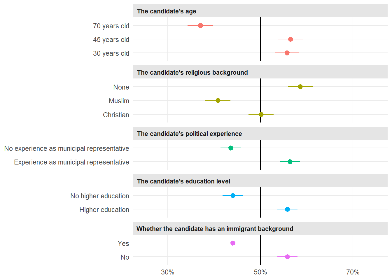
mm_cnd

            term                                     value  estimate  std.error
1        cnd_age                              30 years old 0.5574163 0.01351678
2        cnd_age                              45 years old 0.5652906 0.01389302
3        cnd_age                              70 years old 0.3705628 0.01408416
4        cnd_rel                                 Christian 0.5016639 0.01380606
5        cnd_rel                                    Muslim 0.4080411 0.01399957
6        cnd_rel                                      None 0.5861224 0.01367584
7      cnd_polex    Experience as municipal representative 0.5638889 0.01128199
8      cnd_polex No experience as municipal representative 0.4359688 0.01129455
9        cnd_edu                          Higher education 0.5585635 0.01125078
10       cnd_edu                       No higher education 0.4406495 0.01132612
11 cnd_immigrant                                        No 0.5585635 0.01125078
12 cnd_immigrant                                       Yes 0.4406495 0.01132612
   statistic       p.value  s.value  conf.low conf.high
1   41.23884  0.000000e+00      Inf 0.5309239 0.5839087
2   40.68882  0.000000e+00      Inf 0.5380608 0.5925205
3   26.31060 1.450421e-152 504.3966 0.3429583 0.3981672
4   36.33650 4.293820e-289 957.9350 0.4746045 0.5287233
5   29.14668 9.203101e-187 617.9984 0.3806024 0.4354797
6   42.85825  0.000000e+00      Inf 0.5593183 0.6129266
7   49.98133  0.000000e+00      Inf 0.5417766 0.5860012
8   38.59993  0.000000e+00      Inf 0.4138319 0.4581057
9   49.64664  0.000000e+00      Inf 0.5365124 0.5806147
10  38.90559  0.000000e+00      Inf 0.4184507 0.4628483
11  49.64664  0.000000e+00      Inf 0.5365124 0.5806147
12  38.90559  0.000000e+00      Inf 0.4184507 0.4628483

Code

plot_mm_cnd <- mm_cnd %>% 
  as_tibble() %>% 
  mutate(value = fct_inorder(value)) %>%
  left_join(variable_lookup, by = join_by(term == variable)) %>% 
  mutate(across(c(value, variable_nice), ~fct_inorder(.)))

plot1 <- ggplot(
  plot_mm_cnd,
  aes(x = estimate, y = value, color = variable_nice)
) +
  geom_vline(xintercept = 0.5) +
  geom_pointrange(aes(xmin = conf.low, xmax = conf.high)) +
 scale_x_continuous(limits = c(0.25, 0.75),
                     breaks = c(0.3, 0.5, 0.7),
                    labels = label_percent()) +
  guides(color = "none") +
  labs(
   # title = " ",
    #subtitle = " ",
    x = NULL,
    y = NULL,
    color = "Feature"  ) +
  facet_col(facets = "variable_nice", scales = "free_y", space = "free")

plot1

Code

ggsave(filename = 'electability-citizens-main.png', plot=last_plot(), dpi=300)

Saving 7 x 5 in image

Analysis of Elected Representatives

Code

lm_cnd <- df_long %>%
  filter(dataset_origin == "df_per") %>%   # Filter only df_per respondents
  lm(chosen ~ cnd_age + cnd_rel + cnd_polex + cnd_edu + cnd_immigrant, data = .)

mm_cnd <- marginal_means(
  lm_cnd,
  newdata = c("cnd_age", "cnd_rel", "cnd_polex", "cnd_edu", "cnd_immigrant"),
  wts = "cells"
)
mm_cnd

            term                                     value  estimate
1        cnd_age                              30 years old 0.5098550
2        cnd_age                              45 years old 0.4843690
3        cnd_age                              70 years old 0.5051471
4        cnd_rel                                 Christian 0.5014881
5        cnd_rel                                    Muslim 0.4912018
6        cnd_rel                                      None 0.5073836
7      cnd_polex    Experience as municipal representative 0.4976185
8      cnd_polex No experience as municipal representative 0.5023685
9        cnd_edu                          Higher education 0.4979403
10       cnd_edu                       No higher education 0.5019436
11 cnd_immigrant                                        No 0.4979403
12 cnd_immigrant                                       Yes 0.5019436
     std.error statistic p.value s.value  conf.low conf.high
1  0.009642999  52.87307       0     Inf 0.4909550 0.5287549
2  0.009823671  49.30631       0     Inf 0.4651149 0.5036230
3  0.009587892  52.68594       0     Inf 0.4863551 0.5239390
4  0.009644793  51.99574       0     Inf 0.4825846 0.5203915
5  0.009675439  50.76791       0     Inf 0.4722383 0.5101653
6  0.009730236  52.14504       0     Inf 0.4883127 0.5264545
7  0.007917271  62.85227       0     Inf 0.4821009 0.5131360
8  0.007895529  63.62696       0     Inf 0.4868935 0.5178434
9  0.008023575  62.05965       0     Inf 0.4822143 0.5136662
10 0.007794179  64.39981       0     Inf 0.4866673 0.5172199
11 0.008023575  62.05965       0     Inf 0.4822143 0.5136662
12 0.007794179  64.39981       0     Inf 0.4866673 0.5172199

Code

plot_mm_cnd <- mm_cnd %>% 
  as_tibble() %>% 
  mutate(value = fct_inorder(value)) %>%
  left_join(variable_lookup, by = join_by(term == variable)) %>% 
  mutate(across(c(value, variable_nice), ~fct_inorder(.)))

plot2 <- ggplot(
  plot_mm_cnd,
  aes(x = estimate, y = value, color = variable_nice)
) +
  geom_vline(xintercept = 0.5) +
  geom_pointrange(aes(xmin = conf.low, xmax = conf.high)) +
 scale_x_continuous(limits = c(0.25, 0.75),
                     breaks = c(0.3, 0.5, 0.7),
                    labels = label_percent()) +
  guides(color = "none") +
  labs(
   # title = " ",
    #subtitle = " ",
    x = NULL,
    y = NULL,
    color = "Feature"  ) +
  facet_col(facets = "variable_nice", scales = "free_y", space = "free")

plot2

Code

ggsave(filename = 'electability-politicians-main.png', plot=last_plot(), dpi=300)

Saving 7 x 5 in image

Citizens and Elected Representatives side-by-side

Code

library(patchwork)
spacer <- plot_spacer()  # Empty spacer to create alignment effect

combined_plot <- (plot1 | (spacer / plot2)) +
  plot_layout(heights = c(2, 0.7)) + # This sets plot1 to be twice the width of plot2
   plot_annotation(tag_levels = 'A')

combined_plot

Code

ggsave("combined_plot.png", combined_plot, width = 7.5, height = 5, dpi = 300)

Difference between Citizens and Elected Representatives –>

TBA

Appendix

Data Generating Infrastructure

The data was collected through the Coordinated Online Panels for Research on Democracy and Governance in Norway (KODEM). We fielded the study in two of the infrastructe’s panels: The Norwegian Citizen Panel, and The Panel of Elected Representatives:

The Norwegian Citizen Panel

The Norwegian Citizen Panel is a web-based platform for surveying public opinion on social and political issues in Norway. Established in 2013, it is owned by the University of Bergen, while recruitment, production, and documentation are managed by ideas2evidence. Surveys are conducted three times per year, drawing randomized samples from the Norwegian Population Registry of citizens aged 18 and older. Data is stored and shared by Sikt, ensuring accessible documentation. The 31st wave was fielded from 04.11.2024 to 25.11.2024, with email and text reminders sent to encourage participation. To address sampling bias, a weighting procedure accounts for respondents’ geography, gender, age, and two-part education level. Missing data on education are weighted using only demographic information. Weighted data preserve the total count of respondents, enabling nuanced analysis for both full samples and sub-groups. The Norwegian Citizen Panel invites research proposals for survey content, promoting broad academic collaboration and public knowledge exchange.

Fielding

Data Collection

Responses by mode of contact

The survey was distributed to 29 759 panel members on 4 November 2024 for the softlaunch and 5 November for the main launch. The invitation contained information on the Norwegian Citizen Panel, unique URLs for each panel member that led to the questionnaire, and a unique access code which the panel members could use to log in to the survey by accessing a link on uib.no/medborger.

The invitation, first reminder, and third reminder were all distributed by e-mail. The second reminder was, depending on whether the panel member had a registered mobile phone number, distributed via SMS or e-mail. Prior to wave 31, 53.4 percent of the panel members were registered with a mobile phone number.

Table 2: Responses and response rate for panel members during data collection

Event	Response	Cumulative responses	Response rate	Cumulative response rate
Invitation (4th/5th of November)	5 555	5 555	34.6 %	34.6 %
First reminder (8th of November)	2 806	8 361	17.5 %	52.1 %
Second reminder - email (13th of November)	515	8 876	3.2 %	55.3 %
Second reminder - SMS (13th of November)	1 437	10 313	9 %	64.3 %
Third reminder (19th of November)	1 202	11 515	7.5 %	71.8 %

In total, 11 515 existing panel members filled out the questionnaire. A response rate of 34.6% was achieved between the invitation and the first reminder. Following a pattern observed in previous waves, the initial invitation produced a higher number of respondents than subsequent reminders. See Table 2 for further details on respondent numbers after reminders.

Using the same methodology as in previous waves for calculating response rate, respondents who have not participated in any of the last three waves are excluded. This leaves us with 16 054 eligible respondents. The overall response rate, as reported in Table 2, is 71.8%.

Approximately 1 700 of the initial invitations were reported as not delivered by Confirmit, which amounts to about 5%. Although measures are taken to ensure email deliverability, it is difficult to accurately estimate how many of the delivered emails ended up in recipients’ spam folders.

The Panel of Elected Representatives

The Panel of Elected Representatives (PER) is an internet-based panel of elected representatives, at all political levels, in Norway. The panel is used for academic research dealing with matters that are important to society, representation and democracy. PER was initiated and run by researchers at the University of Bergen, and is now a part of the national KODEM survey infrastructure.

Overview of Experiment Variables - The Panel of Elected Representatives

TBA

Overview of Experiment Variables - The Norwegian Citizen Panel

r31_poelex_religion1

Variable label:
Experiment. Randomly selects religion for candidate A in r31_poelex.

Field period:
04.11.2024 - 25.11.2024

Technical description:
[Randomized if (r31_group = 1) | (r31_group = 2) | (r31_group = 3) | (r31_group = 4)]

[80% of data withheld.]

Technical attributes:
[Question type: Single] [Format: numeric] [Valid: 0] [Invalid: 11515] [Range: -]

---

r31_poelex_religion2

Variable label:
Experiment. Randomly selects religion for candidate B in r31_poelex.

Field period:
04.11.2024 - 25.11.2024

Technical description:
[Randomized if (r31_group = 1) | (r31_group = 2) | (r31_group = 3) | (r31_group = 4)]

[80% of data withheld.]

Technical attributes:
[Question type: Single] [Format: numeric] [Valid: 0] [Invalid: 11515] [Range: -]

r31_poelex_innvandring1

Variable label:
Experiment. Randomly selects immigration status for candidate A in r31_poelex.

Field period:
04.11.2024 - 25.11.2024

Technical description:
[Randomized if (r31_group = 1) | (r31_group = 2) | (r31_group = 3) | (r31_group = 4)]

[80% of data withheld.]

Technical attributes:
[Question type: Single] [Format: numeric] [Valid: 0] [Invalid: 11515] [Range: -]

r31_poelex_innvandring2

Variable label:
Experiment. Randomly selects immigration status for candidate B in r31_poelex.

Field period:
04.11.2024 - 25.11.2024

Technical description:
[Randomized if (r31_group = 1) | (r31_group = 2) | (r31_group = 3) | (r31_group = 4)]

[80% of data withheld.]

Technical attributes:
[Question type: Single] [Format: numeric] [Valid: 0] [Invalid: 11515] [Range: -]

r31_poelex_alder1

Variable label:
Experiment. Randomly selects age for candidate A in r31_poelex.

Field period:
04.11.2024 - 25.11.2024

Technical description:
[Randomized if (r31_group = 1) | (r31_group = 2) | (r31_group = 3) | (r31_group = 4)]

[80% of data withheld.]

Technical attributes:
[Question type: Single] [Format: numeric] [Valid: 0] [Invalid: 11515] [Range: -]

r31_poelex_alder2

Variable label:
Experiment. Randomly selects age for candidate B in r31_poelex.

Field period:
04.11.2024 - 25.11.2024

Technical description:
[Randomized if (r31_group = 1) | (r31_group = 2) | (r31_group = 3) | (r31_group = 4)]

[80% of data withheld.]

Technical attributes:
[Question type: Single] [Format: numeric] [Valid: 0] [Invalid: 11515] [Range: -]

r31_poelex_utd1

Variable label:
Experiment. Randomly selects education level for candidate A in r31_poelex.

Field period:
04.11.2024 - 25.11.2024

Technical description:
[Randomized if (r31_group = 1) | (r31_group = 2) | (r31_group = 3) | (r31_group = 4)]

[80% of data withheld.]

Technical attributes:
[Question type: Single] [Format: numeric] [Valid: 0] [Invalid: 11515] [Range: -]

r31_poelex_utd2

Variable label:
Experiment. Randomly selects education level for candidate B in r31_poelex.

Field period:
04.11.2024 - 25.11.2024

Technical description:
[Randomized if (r31_group = 1) | (r31_group = 2) | (r31_group = 3) | (r31_group = 4)]

[80% of data withheld.]

Technical attributes:
[Question type: Single] [Format: numeric] [Valid: 0] [Invalid: 11515] [Range: -]

r31_poelex_gender1

Variable label:
Experiment. Randomly selects gender for candidate A in r31_poelex.

Field period:
04.11.2024 - 25.11.2024

Technical description:
[Randomized if (r31_group = 1) | (r31_group = 2) | (r31_group = 3) | (r31_group = 4)]

[80% of data withheld.]

Technical attributes:
[Question type: Single] [Format: numeric] [Valid: 0] [Invalid: 11515] [Range: -]

r31_poelex_gender2

Variable label:
Experiment. Randomly selects gender for candidate B in r31_poelex.

Field period:
04.11.2024 - 25.11.2024

Technical description:
[Randomized if (r31_group = 1) | (r31_group = 2) | (r31_group = 3) | (r31_group = 4)]

[80% of data withheld.]

Technical attributes:
[Question type: Single] [Format: numeric] [Valid: 0] [Invalid: 11515] [Range: -]

r31_poelex_polerfaring1

Variable label:
Experiment. Randomly selects political experience for candidate A in r31_poelex.

Field period:
04.11.2024 - 25.11.2024

Technical description:
[Randomized if (r31_group = 1) | (r31_group = 2) | (r31_group = 3) | (r31_group = 4)]

[80% of data withheld.]

Technical attributes:
[Question type: Single] [Format: numeric] [Valid: 0] [Invalid: 11515] [Range: -]

r31_poelex_polerfaring2

Variable label:
Experiment. Randomly selects political experience for candidate B in r31_poelex.

Field period:
04.11.2024 - 25.11.2024

Technical description:
[Randomized if (r31_group = 1) | (r31_group = 2) | (r31_group = 3) | (r31_group = 4)]

[80% of data withheld.]

Technical attributes:
[Question type: Single] [Format: numeric] [Valid: 0] [Invalid: 11515] [Range: -]

r31_poelex_rerandomize

Variable label:
Experiment. Technical details on re-randomisation of r31_poelex-variables if it was necessary.

Field period:
04.11.2024 - 25.11.2024

Technical description:
[If there was a necessity to re-randomise information for one of the candidates in [r30_poelex], the information is stored here.]

[80% of data withheld.]

Technical attributes:
[Question type: Open] [Format: numeric] [Valid: 0] [Invalid: 11515] [Range: -]

r31_poelex_roworder

Variable label:
Experiment. The random order of attributes shown in the table in r31_poelex. Sets the subject’s rowwise placement, sorted by subject.

Field period:
04.11.2024 - 25.11.2024

Technical description:
[If the first number is 2, it means that subject 1 (“religion”) was displayed in row number 2. If the second number is 4, it means that subject 1 (“immigration status”) was displayed in row number 4, etc.
For the sequential order, sorted by rownumber, see r31_poelex_roworder_seq.
1 = Religion. 2 = Immigration status. 3 = Age. 4 = Education level. 5 = Gender. 6 = Political experience.]

[80% of data withheld.]

Technical attributes:
[Question type: Open] [Format: numeric] [Valid: 0] [Invalid: 11515] [Range: -]

r31_poelex_roworder_seq

Variable label:
Experiment. The random order of attributes shown in the table in r31_poelex. Set sequentially, sorted by rownumber.

Field period:
04.11.2024 - 25.11.2024

Technical description:
[The first number in the array shows what category was displayed in the first row, while the next number shows what category was shown in the second row, etc.
1 = Religion. 2 = Immigration status. 3 = Age. 4 = Education level. 5 = Gender. 6 = Political experience.]

[80% of data withheld.]

Technical attributes:
[Question type: Open] [Format: numeric] [Valid: 0] [Invalid: 11515] [Range: -]

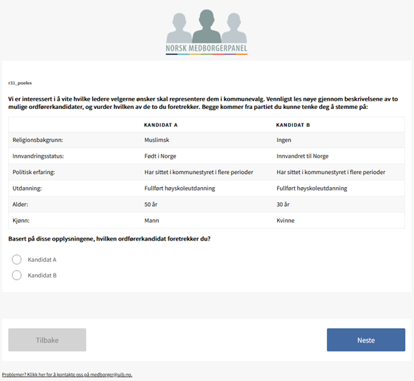
r31_poelex

Variable label:
Preferred mayoral candidate

Literal question:
> We are interested in knowing which leaders voters would like to represent them in the municipal elections. Please read carefully the descriptions about two possible mayoral candidates and consider which of the two you prefer. Both represent the party that you would like to vote for: > > Candidate A r31_poelex_religion1 r31_poelex_innvandring1 r31_poelex_alder1 r31_poelex_utd1 r31_poelex_gender1 r31_poelex_polerfaring1 > > Candidate B r31_poelex_religion2 r31_poelex_innvandring2 r31_poelex_alder2 r31_poelex_utd2 r31_poelex_gender2 r31_poelex_polerfaring2 > > Based on this information, which mayoral candidate do you prefer?

Equivalent in other panels:
p11_poelex

Field period:
04.11.2024 - 25.11.2024

Technical description:
[Asked if (r31_group = 1) | (r31_group = 2) | (r31_group = 3) | (r31_group = 4)]

[Respondents were shown information about the candidates in a table. Variables listed in question text were shown in random order which is stored in r31_poelex_roworder and r31_poelex_roworder_seq.
If [r31_group] = 1, 3 the respondents were exposed to the question after [r31_pceum]. If [r31_group] = 2 the respondents were exposed to the question after [r31_pohpqxc]. If [r31_group] = 4 the respondents were exposed to the question after [r31_dmaicx].]

[80% of data withheld.]

Technical attributes:
[Question type: Single] [Format: numeric] [Valid: 0] [Invalid: 11515] [Range: -]

Screen shot of r31_poelex.png

References

Arnesen, Sveinung, Dominik Duell, and Mikael Poul Johannesson. 2019. “Do Citizens Make Inferences from Political Candidate Characteristics When Aiming for Substantive Representation?” Electoral Studies 57: 46–60.

Brady, Henry, and Paul Sniderman. 1985. “Attitude Attribution: A Group Basis for Political Reasoning.” American Political Science Review 79 (4): 1061–78.

Butler, Daniel M. 2014. Representing the Advantaged: How Politicians Reinforce Inequality. Cambridge University Press.

Carnes, Nicholas. 2012. “Does the Numerical Underrepresentation of the Working Class in Congress Matter?” Legislative Studies Quarterly 37 (1): 5–34.

Carnes, Nicholas, and Noam Lupu. 2023. “The Economic Backgrounds of Politicians.” Annual Review of Political Science 26.

Eshima, Shusei, and Daniel M Smith. 2022. “Just a Number? Voter Evaluations of Age in Candidate-Choice Experiments.” The Journal of Politics 84 (3): 1856–61.

Hainmueller, Jens, Dominik Hangartner, and Teppei Yamamoto. 2015. “Validating Vignette and Conjoint Survey Experiments Against Real-World Behavior.” Proceedings of the National Academy of Sciences 112 (8): 2395–2400.

Hainmueller, Jens, Daniel J Hopkins, and Teppei Yamamoto. 2014. “Causal Inference in Conjoint Analysis: Understanding Multidimensional Choices via Stated Preference Experiments.” Political Analysis 22 (1): 1–30.

Kirkland, Patricia A, and Alexander Coppock. 2018. “Candidate Choice Without Party Labels.” Political Behavior 40 (3): 571–91.

Leeper, Thomas J, Sara B Hobolt, and James Tilley. 2018. “Measuring Subgroup Preferences in Conjoint Experiments.”

Mansbridge, Jane. 1999. “Should Blacks Represent Blacks and Women Represent Women? A Contingent ‘Yes’.” The Journal of Politics 61 (03): 628–57.

Mathisen, Ruben B. 2024. “The Influence Gap: Unequal Policy Responsiveness to Men and Women.” The Journal of Politics 86 (4): 000–000.

McClean, Charles T, and Yoshikuni Ono. 2024. “Too Young to Run? Voter Evaluations of the Age of Candidates.” Political Behavior, 1–23.

Oosten, Sanne van, Liza Mügge, and Daphne van der Pas. 2024. “Race/Ethnicity in Candidate Experiments: A Meta-Analysis and the Case for Shared Identification.” Acta Politica, 19–41. https://doi.org/https://doi.org/10.1057/s41269-022-00279-y.

Schwarz, Susanne, and Alexander Coppock. 2022. “What Have We Learned about Gender from Candidate Choice Experiments? A Meta-Analysis of Sixty-Seven Factorial Survey Experiments.” The Journal of Politics 84 (2): 655–68.

Verba, Sidney, Kay Lehman Schlozman, and Henry Brady. 1995. Voice and Equality: Civic Voluntarism in American Politics. Harvard University Press.