anno_df <- metadata[, c("Id", "long", "lat", "Group")]
colnames(anno_df) <- c("Id", "Longitude", "Latitude", "Group")

sample_map(anno_df, mode = 1, group = "Group", xlim = c(90, 135), ylim = c(20, 50))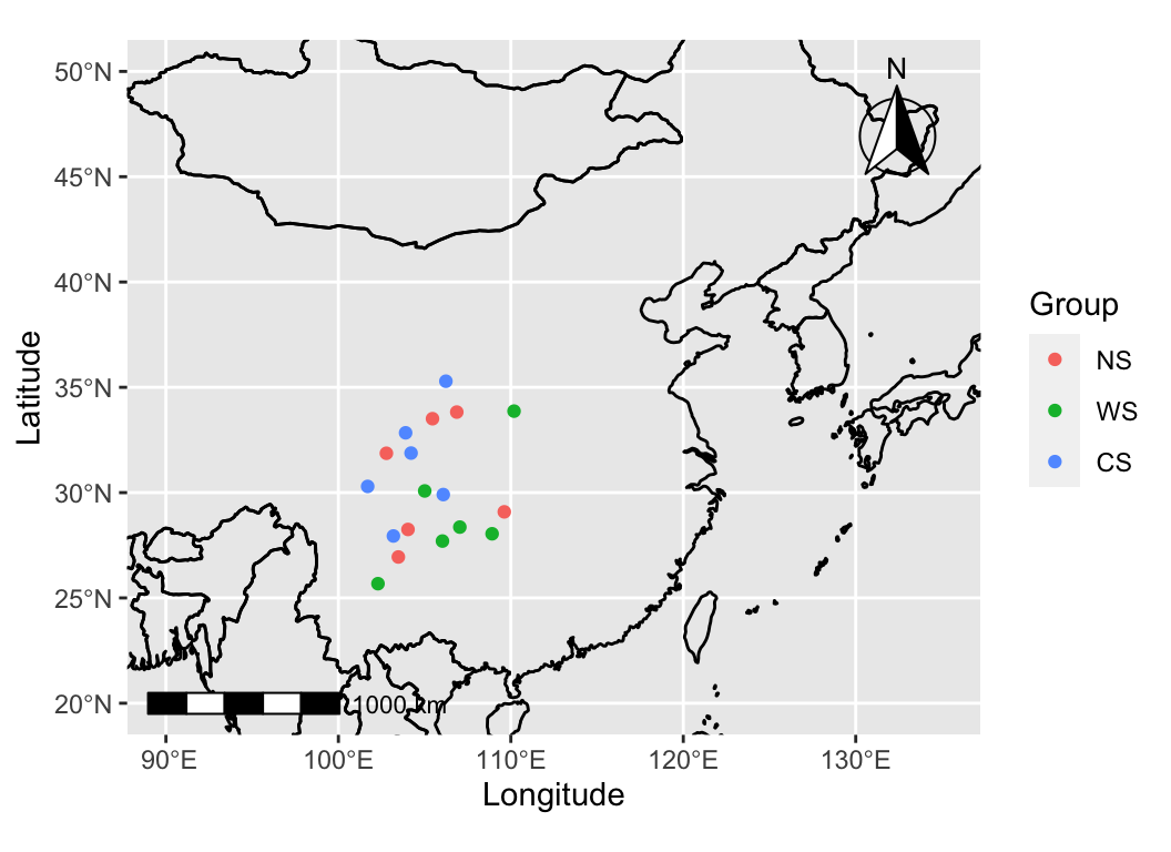
Before delving into the exploration of omics data, a thorough understanding of the metadata is crucial.
If there are well-defined experimental groups, the focus can be on identifying differences between these groups and understanding the sources of these differences, assuming a hypothesis-driven approach.
On the other hand, in the absence of explicit experimental groups but with various environmental factors, one can explore a variety of exploratory analysis methods to uncover interesting patterns or results, following a data-driven research approach.
We often use maps to visualize the sampling locations of our experiments, overlaying important information on the sampling points.
sample_map is a tool that facilitates the quick and convenient creation of various types of sampling maps.
anno_df <- metadata[, c("Id", "long", "lat", "Group")]
colnames(anno_df) <- c("Id", "Longitude", "Latitude", "Group")
sample_map(anno_df, mode = 1, group = "Group", xlim = c(90, 135), ylim = c(20, 50))sample_map(anno_df, mode = 3, group = "Group")For more details on creating maps in R, you can refer to Plot beautiful maps with R.
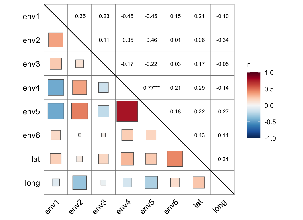
cor_plot(metadata[, 3:10])
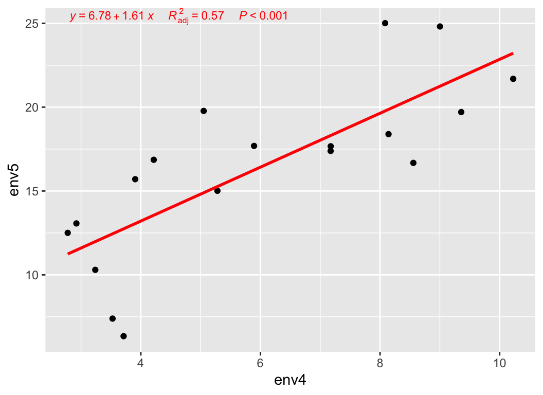
my_lm(metadata["env5"], var = "env4", metadata)
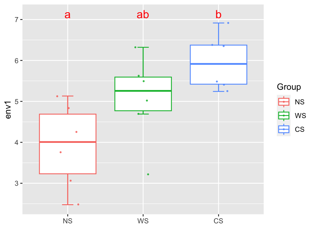
group_box(metadata["env1"], group = "Group", metadata, alpha = T)
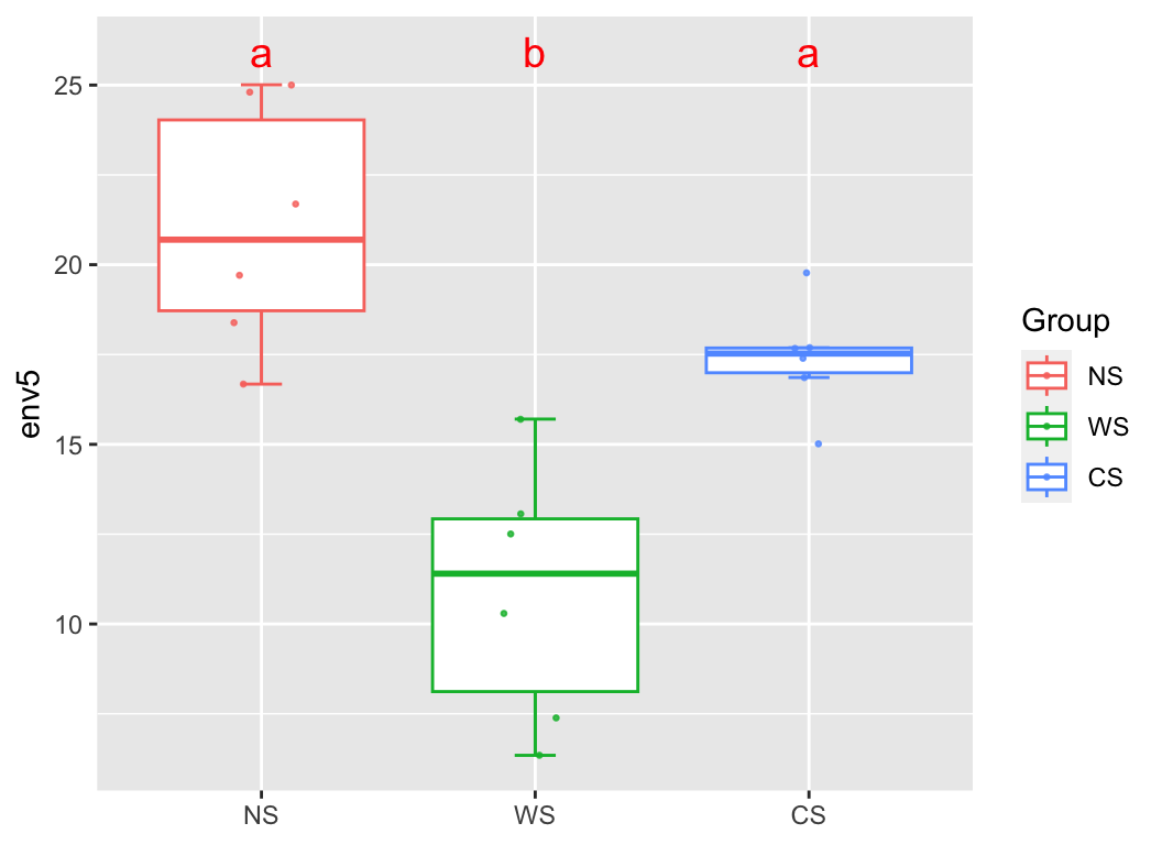
group_box(metadata["env5"], group = "Group", metadata, alpha = T)