Chapter 6 Making your first Reproducible Document

Figure 6.1: RMarkdown by Allison Horst

This chapter is what makes your entire workflow sync.

There are several possible output formats that your RMarkdown file can render. They each have their subleties which are outside the scope of this book. PDF and HTML allow for the greatest customizability however, in academia I have found Microsoft Word is king. Your advisor, colleagues they all use it. So I am not going to attempt to re-invent the wheel here which is why we are knitting to *.docx. I am going to give you the essentials that you need to get started, that being said, there is a whole universe for you left to explore beyond this course if you so desire. There is a very strong argument to export using LaTEX, but in my experience most research teams are unfamiliar with LaTEX. For this reason, I prefer to use docx. If you do use a LaTEX environment it is easier to customize than docx and also has stronger background with templates (see the rticles packages).

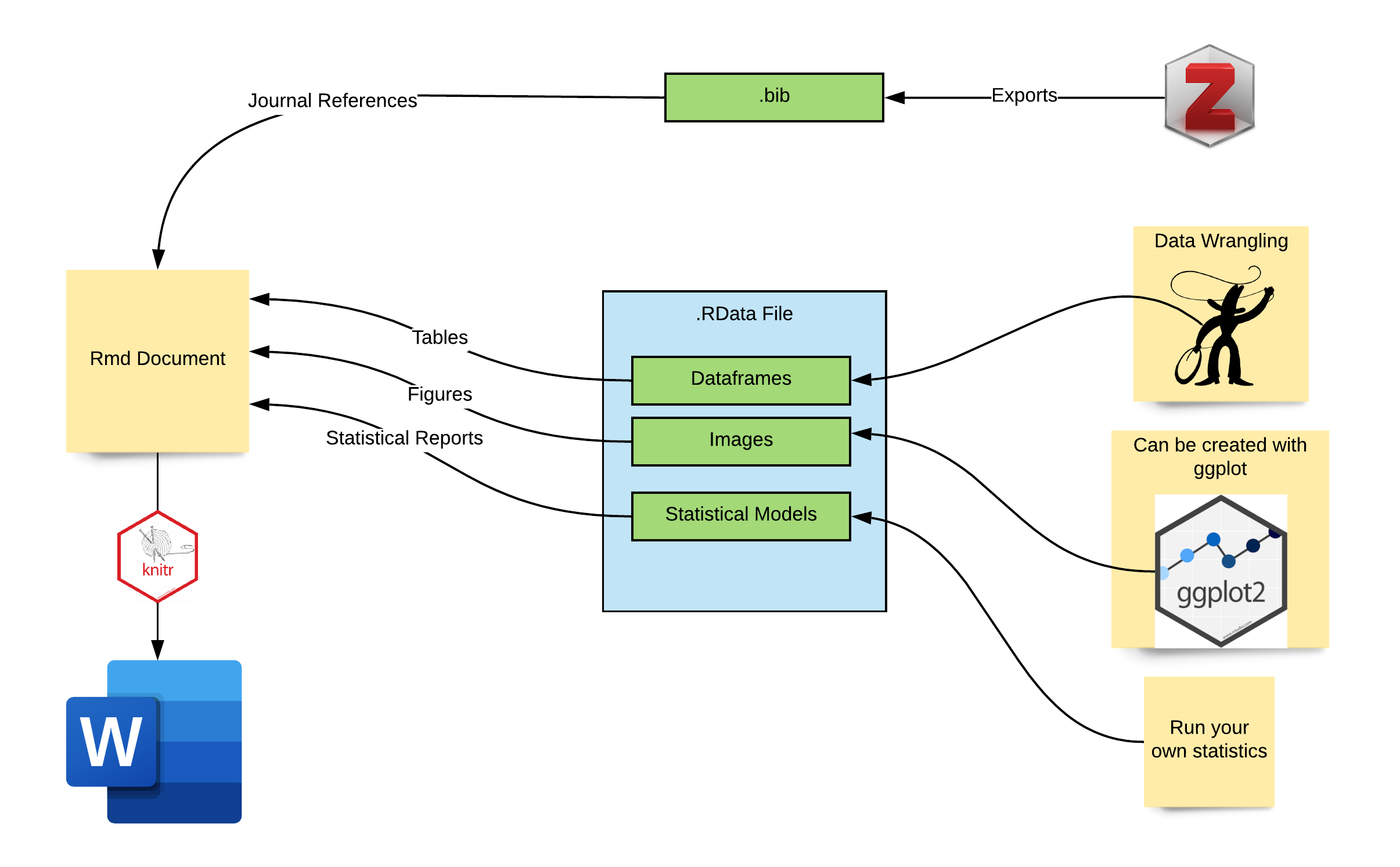
Figure 6.2: RMarkdown Outputs

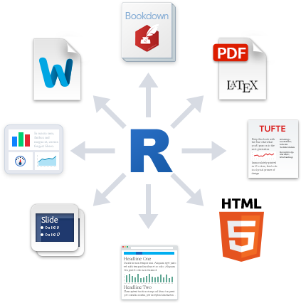
Figure 6.3: RMarkdown Outputs

See here

6.1 What goes into an Rmd document??

To answer this question effectively, we first need to consider what goes into a typical manuscript. Below is an illustration. As you can see, we have four main components:

Tables
Figures
Citations
Statistical results

We are going to go through each of these step by step in the next few headers.

6.2 Example Reproducible Document

This section assumes you have downloaded MyProjectName folder on your computer.

6.3 YAML Explained

YAML is the first part of code in your *.Rmd document. It controls how your document will be compiled. BE CAREFUL YAML is space and case sensitive.

Within YAML we find a few key components which we will go over now.

Insert your name Insert your project name Insert the path to your .bib file Change the .csl file to another format

6.3.1 Citations

Here we assume you have Zotero installed and you have exported your library. In the mean time you can use the one provided to you from my current project directory. Below in Figure 6.4 is an illustration of how citations work. There are two important files

.bib file which contains your references
.csl file which handles the formatting in-text

Before we get too far….mess around with YAML.

Insert your name Insert your project name Insert the path to your .bib file Change the .csl file to another format

knitr::include_graphics("images/bookdown_elements/RMarkdown-Citations.png")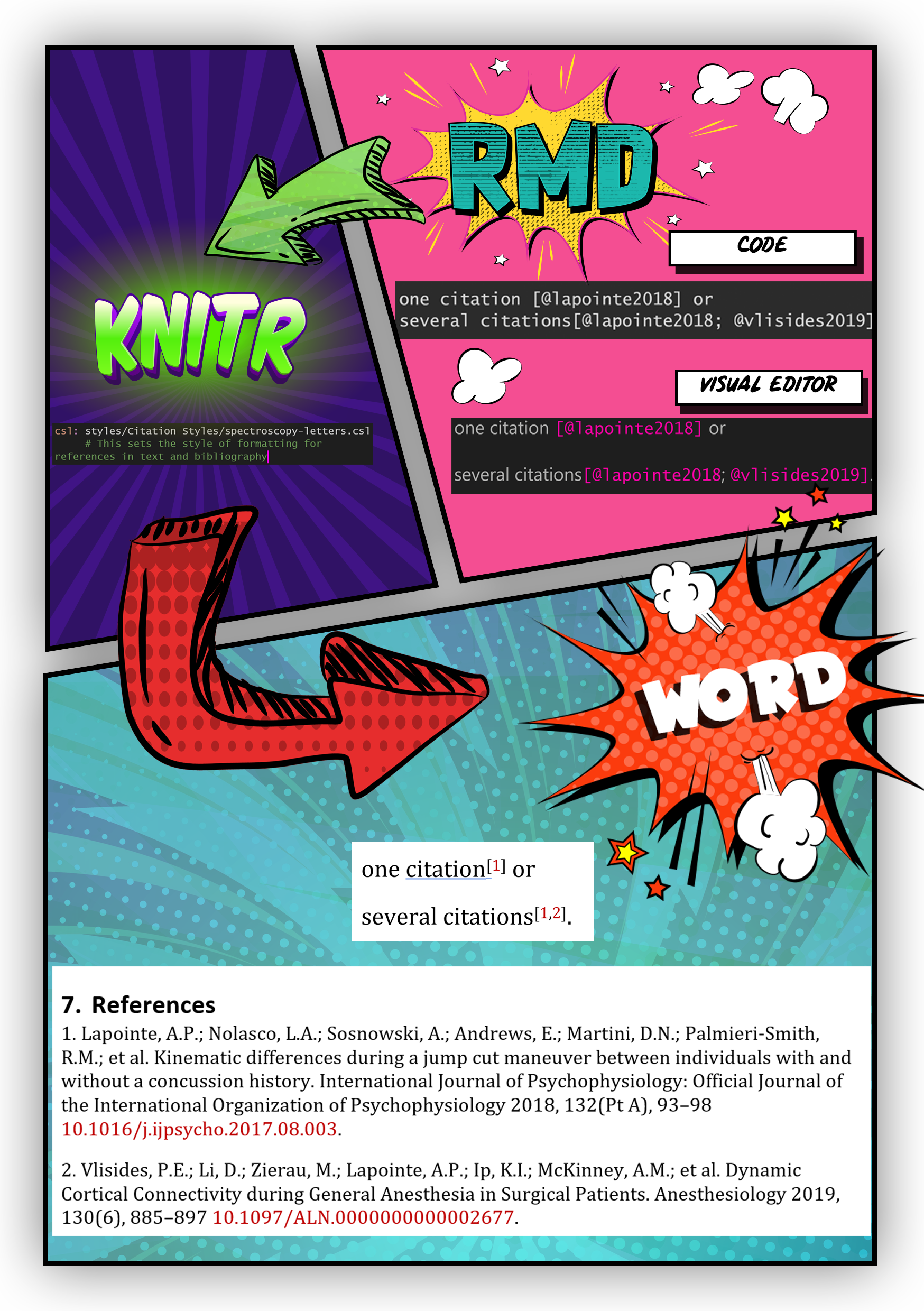

Figure 6.4: Citations in RMarkdown

Import a new citation into Zotero Add that citation into your Rmd document

6.4 Referencing a Figure

Figures can be inserted using a similar workflow. In Figure 6.5 is an illustration of how figures work

knitr::include_graphics("images/bookdown_elements/RMarkdown-Figures.png")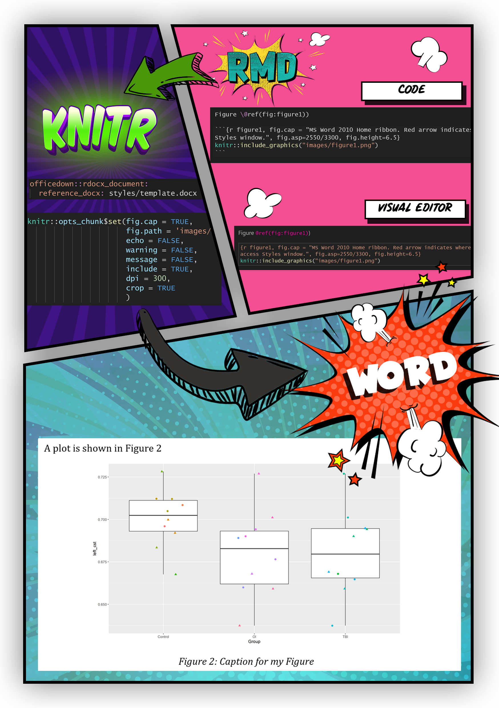

Figure 6.5: Figures in RMarkdown

Notice how in the body of your Rmd document there is a code reference which gets called within your knitr chunk. There are a few rules when naming this code reference

✅ dashes
- \@ref(fig:my-awesome-table)
⛔ spaces
- \@ref(fig:myawesometable)
⛔ underscores
- \@ref(fig:my_awesome_table)
⛔ periods
- \@ref(fig:my.awesome.table)

A plot is shown in Figure \@ref(fig:myFigure1)

knitr::include_graphics("images/plot1.png")

6.4.1 Chunk Options/Elements

The first element that gets called is your code reference, followed by your desired caption in fig.cap.

Download an image off the internet Store it in /images folder Add a new reference and chunk in manuscript.Rmd Re-knit the document

6.5 Referencing a table

Tables work very similarly to figures

Descriptive statistics were run and are shown in Table \@ref(tab:journeyTime2) below

knitr::kable(iris, longtable=T, caption = "Descriptives")

Go into Excel and create a simple dataset Save it in /data folder Insert your own table into the Rmd
Re-knit the document

6.5.1 Results

For more in-depth description of other functions you can use in text I would go to the apastats folder on your computer R\win-library\4.0\apastats\html which will show a list of html files with descriptions.

There was a significant effect of service on the average journey time

r describe.aov(model, "service", sstype = 2)

6.5.2 In text statistics

This is common when describing demographics within an article. An example would be

“A convenience sample of 10 healthy controls (6 females, 4 males) aged XX ± YY years”

The value “XX” and “YY” can be replaced with code, such that if ever we update our dataset, this values get automatically updated.

# Raw syntax without the Visual Editor
A convenience sample of 10 healthy controls (6 females, 4 males) aged `r round(mean(tbl.demographics$Age),1)` ± `r round(sd(tbl.demographics$Age),1)` years

knitr::include_graphics("https://i.imgur.com/4gdQ1kQ.png")

knitr::include_graphics("https://i.imgur.com/uIE5aV1.png")

6.5.3 Equations

Equation in RMarkdown use LaTeX encoding. I would recommend using a LaTeX equation maker online and pasting the code into your document. Here is an example.

6.6 Creating your own Word Template

Perhaps you don’t like the look of your current document. That’s ok!! Much of the formatting of your document is handled by a reference document, a template which knitr emulates when it renders your document. We can modify current styles and even create some * Create an MS Word Template for RMarkdown

6.7 Writing

Notice how headers are denoted using the # symbol.

6.8 Other operations


## Advanced Code 

### Moving the Reference section before the end of the document
In some of my manuscript submissions I want the **References** section to show up before the end of the document. This can be accomplished using this code snippet


```r
\newpage
# References {-}
<div id="refs"></div>
\newpage

6.8.1 Table of Content, Figures and Tables.

In order to add these elements at the beginning of your document use the following code with the officedown and officer packages

## Table of content

<!---BLOCK_TOC--->

## List of figures

<!---BLOCK_TOC{seq_id: 'fig'}--->

## List of tables

<!---BLOCK_TOC{seq_id: 'tab'}--->

6.8.2 Having a separate numbering for Supplementary Materials

I ran into this issue where I needed the numbering to restart in Supplementary Figures. You can view my complete answer and reproducible example on StackOverflow