5 Intro to R using R Markdown
In this chapter, you’ll see many of the ways that R stores objects and more details on how you can use functions to solve problems in R. You’ll be working with a common dataset derived from something that you likely have encountered before: the periodic table from chemistry.
5.1 A beginning directory/file workflow
“File organization and naming are powerful weapons against chaos.” - Jenny Bryan
Something that is not frequently discussed when working with files and programming languages like R is the importance of naming your files something relevantly and having organization of your files in folders. You may be tempted to call a file analysis.Rmd but what happens when you need to change your analysis months from now and you’ve named many files for many different projects analysis.Rmd in many different folders. It’s much better to give your future self a break and commit to concise naming strategies.
You can choose a variety of ways to name files. These guidelines are what I try to follow:
Group similar style files into the same folder whenever possible.
Try not to have one folder that contains all of the different types of files you are working with. It is much easier to find what you are looking for if you put all of your
datafiles in adatafolder, all of yourfigurefiles in afigurefolder, and so on.This rule can be broken if you only have one or two of each type. It can be the case that too many folders can waste your time when a useful search for the appropriate file may be able to find your file faster than digging through a complex hierarchy of directories.
Name your files consistently so that what the file contains can be easily identified from the name of your file, but be concise.
Seeing
test1.Rmdandtest2.Rmddoesn’t tell us much about what is actually in the files. It’s OK to create a temporary file or two if you don’t think you will be using it going forward, but you should be in the habit of reviewing your work at the end of your session and naming files that we needed appropriately.
Something likemodel_fit_sodium.Rmdis so much better in the long-run.
Remember to think about your future self whenever you can, especially with programming. Be nice to yourself so that future self really appreciates past self.Use an underscore to separate elements of the file name.
The underscore
_produces a visually appealing way for us to realize there is a separation between content. You may be tempted to just use a space, but spaces cause problems in R and in other programming languages. Some folks prefer to just change the case of the first letter of the word to bring attention. Here are a few examples of file names. You can be the judge as to what is most appealing to you:barplot_weight_height.RmdvsbarplotWeightHeight.Rmdvsbarplotweightheight.RmdWhatever you choose for style, be consistent and think about other users as you name your files. If you were passed a smorgasbord of files that is a mess to deal with and hard to understand, you wouldn’t like it, right? Don’t be that person to someone else (or yourself)!
5.2 Using R with periodic table dataset
We now hop into the basics of working with a dataset in R. We will also explore the ways R stores data in objects, how to access specific elements in those objects, and also how to use functions, which are one of the most useful pieces of R to help with organization and clean code.
It is worthy to note that many of the functions here such as table and concepts like subsetting, indexing, and creating/modifying new variables can also be done using the great packages that Hadley Wickham has developed and in particular the dplyr package. It is still important to get a sense for how R stores objects and how to interact with objects in the “old-school” way. You’ll still find some times where doing it this old way actually works just as nicely as the newer modern ways…but they are becoming fewer and fewer by the day. Anyways, you’ll hopefully be well-ready to hop into some statistical analyses or data tasks after you follow along with this introduction to R.
5.2.1 Loading data from a file
One of the most common ways you’ll want to work with data is by importing it from a file. A common file format that works nicely with R is the CSV (comma-separated values) file. The following R commands first download the CSV file from the internet on my webpage into the periodic-table-data.csv file on your computer, then reads in the CSV stored, and then gives the name periodic_table to the data frame that stores these values in R:
download.file(url = "http://ismayc.github.io/periodic-table-data.csv",
  destfile = "periodic-table-data.csv")
periodic_table <- read.csv("periodic-table-data.csv",
stringsAsFactors = FALSE)We will be discussing both strings and factors in the data structures section (Section 5.3) and why this additional parameter stringsAsFactors set to FALSE is recommended.
It’s good practice to check out the data after you have loaded it in:
View(periodic_table)The GIF below walks through downloading the CSV file and loading it into the data frame object named periodic_table. In addition, it shows another way to view data frames that is built into RStudio without having to run the View function. Note that a new R Markdown file is created here as well called chemistry_example.Rmd. We are writing the commands directly into R chunks here, but you may find it nicer to play around in your R Console sandbox first.
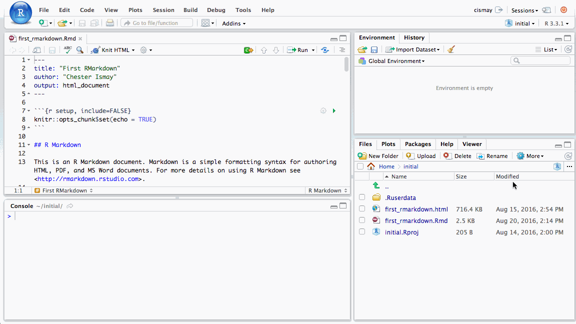
Figure 5.1: Viewing the periodic table data frame
I encourage you to take the R chunks that follow in this chapter, type/copy them into an R Markdown file that has loaded the periodic_table data set, and watch that your resulting output will match the output that I have presented for you here in this book. This book was written in R Markdown after all!
5.3 Data structures
5.3.1 Data frames
Data frames are by far the most common type of object you will work with in R. This makes sense since R is a statistical computing language at its core, so handling spreadsheet-like data is something it should be good at. The periodic_table data set is stored as a data frame. As you can see there are many different types of variables in this data set. We can get a glimpse as to the types and some of the values of the variables by using the str function in the R Console:
str(periodic_table)Each of the names of the variables/columns in the data frame are listed immediately after the $. Then on each row of the str function call after the : we see what type of variable it is. For this periodic_table data set, we have four types: int, chr, num, and logi:
intcorresponds to integer valueschrcorresponds to character string valuesnumcorresponds to numeric (not necessarily integer) valueslogicorresponds to logical values (TRUEorFALSE)
5.3.2 Vectors
Data frames are most commonly just many vectors put together into a single object. Our periodic_table data frame has each row correspond to a chemical element and each column correspond to a different measurement or characteristic of that element. There are many different ways to create a vector that stands on its own outside of a data frame.
Using the c function
If you would like to list out many entries and put them into a vector object, you can do so via the c function. If you enter ?c in the R Console, you can gain information about it. The “c” stands for combine or concatenate.
Suppose we wanted to create a way to store four names:
friend_names <- c("Bertha", "Herbert", "Alice", "Nathaniel")
friend_names
## [1] "Bertha" "Herbert" "Alice" "Nathaniel"You can see when friend_names is outputted that there are four entries to it. This is vector is known as a strings vector since it contains character strings. You can check to see what type an object is by using the class function:
class(friend_names)## [1] "character"Next suppose we wanted to put the ages of our friends in another vector. We can again use the c function:
friend_ages <- c(25L, 37L, 22L, 30L)
friend_ages
## [1] 25 37 22 30class(friend_ages)## [1] "integer"Note the use of the L value here. This tells R that the numbers entered have no decimal components. If we didn’t designate the L we can see that the values are read in as "numeric" by default:
ages_numeric <- c(25, 37, 22, 30)
class(ages_numeric)
## [1] "numeric"There is not a huge difference in how these values are stored from a user’s perspective, but it is a good habit to specify what class your variables are whenever possible to help with collaboration and documentation.
Using the seq function
The most likely way you will enter character values into a vector is via the c function. Numeric values can be entered in a couple different ways. You saw the first way using the c function above. Since numbers have an ordering to them, we can also specify a sequence of numbers with some starting value, ending value, and how much we’d like to increment each step in the sequence:
sequence_by_2 <- seq(from = 0L, to = 100L, by = 2L)
sequence_by_2
## [1] 0 2 4 6 8 10 12 14 16 18 20 22 24 26 28 30 32
## [18] 34 36 38 40 42 44 46 48 50 52 54 56 58 60 62 64 66
## [35] 68 70 72 74 76 78 80 82 84 86 88 90 92 94 96 98 100class(sequence_by_2)## [1] "integer"You now might have a better sense to what the numbers in the [ ] before the output refer to. This is done to help you keep track of where you are in the printing of the output. So the first element denoted by [1] is 0, the 18th entry ([18]) is 34, and the 35th entry ([35]) is 68. This will serve as a nice introduction into indexing and subsetting in Section 5.5.
We can also set the sequence to go by a negative number or a decimal value. We will do both in the next example.
dec_frac_seq <- seq(from = 10, to = 3, by = -0.2)
dec_frac_seq
## [1] 10.0 9.8 9.6 9.4 9.2 9.0 8.8 8.6 8.4 8.2 8.0 7.8 7.6
## [14] 7.4 7.2 7.0 6.8 6.6 6.4 6.2 6.0 5.8 5.6 5.4 5.2 5.0
## [27] 4.8 4.6 4.4 4.2 4.0 3.8 3.6 3.4 3.2 3.0class(dec_frac_seq)## [1] "numeric"Using the : operator
A short-cut version of the seq version can be achieved using the : operator. If we are increasing values by 1 (or -1), we can use the : operator to build our vector:
inc_seq <- 98:112
inc_seq
## [1] 98 99 100 101 102 103 104 105 106 107 108 109 110 111 112dec_seq <- 5:-5
dec_seq## [1] 5 4 3 2 1 0 -1 -2 -3 -4 -5Combining vectors into data frames
If you aren’t reading in data from a file and you have some vectors of information you’d like combined into a single data frame, you can use the data.frame function to do so:
friends <- data.frame(names = friend_names,
                      ages = friend_ages,
                      stringsAsFactors = FALSE)
friends
## names ages
## 1 Bertha 25
## 2 Herbert 37
## 3 Alice 22
## 4 Nathaniel 30Here we have created a names variable in the friends data frame that corresponds to the values in the friend_names vector and similarly an ages variable in friends that corresponds to the values in friend_ages.
5.3.3 Factors
If we have a strings vector/variable that has some sort of natural ordering to it, it frequently makes sense to convert that vector/variable into a factor. The factor will convert the strings to integers to keep track of which order you’d prefer and also keep track of the original string values as well.
Looking over our periodic_table data frame again via View(periodic_table), you can see some good candidates for shifting from chr to Factor. If you remember your chemistry, you’ll know that the natural ordering of the block variable is "s", "p", "d", and "f".
By default, R will organize character strings in alphabetical order. To see this, we’ll introduce two new features: the table function and the $ operator.
table(periodic_table$block)##
## d f p s
## 40 28 36 14We see here a count of the number of elements that appear in each block. But as I said, the ordering is off. You may remember the $ as appearing before the variable names in the str function. That wasn’t a coincidence. To access specific variables inside a data frame we can do so by entering the name of the data frame followed by $ and lastly by the name of the variable. (Note here that spaces in variable names will not work. You’ll learn that the hard way as I have more than likely.)
To convert block into a factor, we use the aptly named factor function. Note that this is “converting” by assigning the result of factor back to block in periodic_table.
periodic_table$block <- factor(periodic_table$block,
levels = c("s", "p", "d", "f"))table(periodic_table$block)##
## s p d f
## 14 36 40 28You’ll find that this is an easy way to organize your data whenever you’d like to summarize it or to plot it, but we’ll save that discussion for a different time and a different book.
5.4 Vectorized operations
R can work extremely quickly when handed a vector or a collection of vectors like a data frame. Instead of walking through each element to perform an operation that we might need to do in other older programming languages, we can do something like this:
five_years_older <- ages_numeric + 5L
five_years_older
## [1] 30 42 27 35Like that, we have ages that are five more than where we started. This extends to adding two vectors together3.
5.5 Indexing and subsetting
So we have a big data frame of information about the periodic table, but what if we wanted to extract smaller pieces of the data frame? You already saw that to focus on any specific variable we can use the $ operator.
5.5.1 Using [ ] with a vector/variable
Recall the use of [ ] when a vector was printed to help us better understand where we are in printing a large vector. We will use this same tool to select the tenth to the twentieth elements of the periodic_table$name variable:
periodic_table$name[10:20]## [1] "Neon" "Sodium" "Magnesium" "Aluminium" "Silicon"
## [6] "Phosphorus" "Sulfur" "Chlorine" "Argon" "Potassium"
## [11] "Calcium"Similarly if we’d only like to select a few elements from our friend_names vector, we can specify the entries directly:
friend_names[c(1, 3)]## [1] "Bertha" "Alice"We can also use - to select everything but the elements listed after it:
friend_names[-c(2, 4)]## [1] "Bertha" "Alice"5.5.2 Using [ , ] with a data frame
We have now seen how to select specific elements of a vector or a variable but what if we wanted a subset of the values in the larger data frame across both rows (observations) and columns (variables). We can use [ , ] where the spot before the comma corresponds to rows and the spot after the comma corresponds to columns. Let’s pick rows 40 to 50 and columns 1, 2, and 4 from periodic_table:
periodic_table[41:50, c(1, 2, 4)]## atomic_number symbol
## 41 41 Nb
## 42 42 Mo
## 43 43 Tc
## 44 44 Ru
## 45 45 Rh
## 46 46 Pd
## 47 47 Ag
## 48 48 Cd
## 49 49 In
## 50 50 Sn
## name_origin
## 41 Niobe, daughter of king Tantalus from Greek mythology
## 42 the Greek molybdos meaning 'lead'
## 43 the Greek tekhn??tos meaning 'artificial'
## 44 Ruthenia, the New Latin name for Russia
## 45 the Greek rhodos, meaning 'rose coloured'
## 46 the then recently discovered asteroid Pallas, considered a planet at the time
## 47 English word (argentum in Latin)
## 48 the New Latin cadmia, from King Kadmos
## 49 indigo
## 50 English word (stannum in Latin)5.5.3 Using logicals
As you’ve seen we can specify directly which elements we’d like to select based on the integer values of the indices of the data frame. Another way to select elements is by using a logical vector:
friend_names[c(TRUE, FALSE, TRUE, FALSE)]## [1] "Bertha" "Alice"This can be extended to choose specific elements from a data frame based on the values in the “cells” of the data frame. A logical vector like the one above (c(TRUE, FALSE, TRUE, FALSE)) can be generated based on our entries:
friend_names == "Bertha"## [1] TRUE FALSE FALSE FALSEWe see that only the first element is set to TRUE as we suspected since "Bertha" is the first entry in the vector. We, thus, have another way of subsetting to choose only those names that are "Bertha" or "Alice":
friend_names[friend_names %in% c("Bertha", "Alice")]## [1] "Bertha" "Alice"The %in% operator looks element-wise in the friend_names vector and then tries to match each entry with the entries in c("Bertha", "Alice").
Now we can think about how to subset an entire data frame using the same sort of creation of two logical vectors (one for rows and one for columns):
periodic_table[ (periodic_table$name %in% c("Hydrogen", "Oxygen") ),
                c("atomic_weight", "state_at_stp")]
## atomic_weight state_at_stp
## 1 1.008235 Gas
## 8 15.999000 GasThe extra parentheses around periodic_table$name %in% c("Hydrogen", "Oxygen") are a good habit to get into as they ensure everything before the comma is used to select specific rows matching that condition. For the columns, we can specify a vector of the column names to focus on only those variables. The resulting table here gives the atomic_weight and state_at_stp for "Hydrogen" and then for "Oxygen".
There are many more complicated ways to subset a data frame and one can use the subset function built into R, but in my experience it is even easier to use the filter and select function in the dplyr package whenever you want to do anything more complicated than what we have done here.
5.6 Functions
We’ve been using functions throughout this entire chapter and you might not have even noticed it. The seq command we saw earlier is a function. It expects a few arguments: from, to, by, and a few others that we didn’t specify. How do I know this and why didn’t we specify them?
Recall that you can look up the help documentation on any function by entering ? and the function name in the R console. If we do this for seq with ?seq, we are given some examples of what to expect under the Usage section. R allows for function arguments to take on default values and that’s what we see:
seq(from = 1, to = 1, by = ((to - from)/(length.out - 1)),
    length.out = NULL, along.with = NULL, ...)
By default, the sequence will both start and end at 1 (a not very interesting sequence). The length.out and along.with arguments are specified to NULL by default. NULL represents an empty object in R, so they are essentially ignored unless the person using the seq function specifies values for them. The ... argument is beyond the scope of this book but you can read more about it and other useful tips about writing function at the NiceRCode page here.
Not all functions have all default arguments like seq. The mean function is one such example:
mean()Error in mean.default() : argument "x" is missing, with no default
Calls: <Anonymous> ... withVisible -> eval -> eval -> mean -> mean.default
Execution halted
Exited with status 1.Notice that an error is given here, where one is not given if you don’t specify the arguments to seq:
seq()## [1] 1To fix the error, we’ll need to specify which vector/object we’d like to compute the mean of. Recall the ages_numeric vector. We can pass that into the mean function:
ages_numeric## [1] 25 37 22 30mean(x = ages_numeric)## [1] 28.5We can also skip specifying the name of the argument if you follow the same order as what is given in Usage in the documentation:
mean(ages_numeric)## [1] 28.5We can see that R expects the arguments to be x, then trim, and then na.rm. What happens if we try to specify TRUE for na.rm without specifically saying na.rm = TRUE?
mean(ages_numeric, TRUE)Error in mean.default(ages_numeric, TRUE) :
'trim' must be numeric of length one
Calls: <Anonymous> ... withVisible -> eval -> eval -> mean -> mean.default
Execution halted
Exited with status 1.Since trim comes before na.rm in the list if we don’t specify our name it will think the second argument is for trim. trim expects a fraction between 0 and 0.5 though so R barks at us that it doesn’t understand. It usually is good practice for beginners to enter the name of the argument and then an equals sign and then the value you’d like the argument to take on. Something like what follows is clean and helps with readability:
mean(x = ages_numeric, na.rm = TRUE)## [1] 28.5Why do some arguments require quotations and others don’t?
As you begin to explore help documentation for different functions, you’ll begin to notice that some arguments require quotations around them while others (like those for mean don’t). This brings us back to the discussion earlier about strings, logicals, and numeric/integer classes.
An example of a function requiring a character string (or vector) is the install.packages function, which is at the heart of R’s ability to expand on its built-in functionality by importing packages that include functions, templates, and data and are written by users of R. If you run ?install.packages you’ll see that the first argument pkgs is expected to be a character vector. You’ll therefore need to enter the packages you’d like to download and install inside quotes.
Two useful packages that I recommend you install and download are "ggplot2" and "dplyr". (Hopefully your instructor/server administrator has already done so for you if you are using an RStudio Server.) This function has a large number of arguments with all but pkgs set by default. We’ll pick a couple here to specify instead of using the defaults:
install.packages(pkgs = c("ggplot2","dplyr"),
                 repos = "http://cran.rstudio.org",
                 dependencies = TRUE,
                 quiet = TRUE)
You’ll notice looking through the help via ?install.packages that what type of argument is expected is given:
pkgsexpects a character vectorreposexpects a character vectordependenciesexpects a logical value (TRUEorFALSE)quietexpects a logical value
After you’ve downloaded the packages, you’ll need to load the package into your R environment using the library function:
library("ggplot2")
library("dplyr")
5.7 Closing thoughts
There are plenty more advanced analyses to be done with R. This chapter serves as a way to get you started with R without digging in too much. I encourage you to review this chapter frequently as you learn to use R. Quiz yourself on what a specific command does and see if you are correct. Breaking R is a pretty hard thing to do. Play around and try to figure out error messages on your own first for 15 minutes or so. If you are still not sure what is going on, check out some of the help with errors in the next chapter.
Vectors of the same size, of course…well, actually R has a way of dealing with vectors of different sizes and not giving errors, but let’s ignore that for now.↩