Chapter 1 Principal Component Analysis
The goal of principal component analysis (PCA) is to project observed data onto a subspace of some chosen dimension \(r\) such that the variability of the projected data is maximised. Alternatively stated, the technique aims to reduce the dimension of each points in the dataset with minimal loss of information. Benefits of PCA include
can identify important features and patterns in the data;
reduction of noise in the dataset;
can improve computing efficiency when working with the dataset;
permits visualisation if dataset reduced to dimension 2 or 3;
can improve interpretability of models fitted to data;
Before one can discuss the mathematics of principal component analysis, one must cover necessary preliminary material: mean-centering and sample covariance, projections, and spectral decomposition.
1.1 Mean-Centering and Sample Covariance Matrix
Consider datapoints \(\mathbf{x}_1, \mathbf{x}_2, \ldots, \mathbf{x}_n\) where \(\mathbf{x}_k \in \mathbb{R}^p\) is a column vector where each entry corresponds to one of the variables or features being observed. Define a matrix \[\mathbf{X} = \begin{pmatrix} \mathbf{x}^T_1 \\ \mathbf{x}^T_2 \\ \vdots \\ \mathbf{x}^T_n \end{pmatrix}.\] where clearly each row of \(\mathbf{X}\) corresponds to one of the observed datapoint. This is a notation for data that we will use throughout the entirety of the module. The sample mean of each feature can be calculated in the vector \(\bar{\mathbf{x}} = \frac{1}{n} \sum\limits_{k=1}^n x_k\).
Set \(\mathbf{1}_n\) to be the \(n \times 1\) column vector of ones, and \(\mathbf{I}_n\) to be the \(n\times n\) identity matrix.
The matrix \(\mathbf{C} = \mathbf{I}_n - \frac{1}{n} \mathbf{1}_n \mathbf{1}_n^T\) is called the centering matrix.
By pre-multiplying the data matrix \(\mathbf{X}\) by \(C\) one obtains the mean-centred data matrix: \[\mathbf{X}_\mathbf{C} = \mathbf{CX} = \mathbf{X} - \mathbf{1}_n \bar{\mathbf{x}} = \begin{pmatrix} \left( \mathbf{x}_1 - \bar{\mathbf{x}}\right)^T \\ \left( \mathbf{x}_2 - \bar{\mathbf{x}}\right)^T \\ \vdots \\ \left( \mathbf{x}_n - \bar{\mathbf{x}} \right)^T \end{pmatrix}\]
That is, pre-multiplying by the centering matrix is equivalent to subtracting the mean from each datapoint. Alternatively by supposing all data has been centered, without loss of generality one can assume that the data has mean \(\mathbf{0}\).
Another important statistic for observed data is that of variance and covariance. Recall that for two random variables \(Z\) and \(Z'\) from which observations \(z_1,\ldots, z_n\) and \(z'_1, \ldots, z'_n\) have been sampled respectively, then the sample covariance is given by \(s_{Z,Z'} = \frac{1}{n} \sum\limits_{k=1}^{n} (z_k - \bar{z})(z'_k - \bar{z'})\). In the case when the observations are assumed to be centered, the formula reduces to \(s_{Z,Z'} = \frac{1}{n} \sum\limits_{k=1}^{n} z_k z'_k\).
It follows from this formula for the sample covariance of centered data that the matrix \(\mathbf{S} = \frac{1}{n} \mathbf{X}_{\mathbf{C}}^T \mathbf{X}_{\mathbf{C}}\) has an entry in the \((i,j)^{th}\) position equal to the sample covariance between the \(i^{th}\) and \(j^{th}\) features of the data. For this reason the matrix \(\mathbf{S}\) is known as the sample covariance matrix.
The following example illustrates how these statistics can be calculated using R.
Consider the data stored in a R dataframe by the following code. Specifically there are three variables x,y,z and seven observations.
df <- data.frame(x = c(1, 4, 5, 6, 6, 8, 9),
                 y = c(7, 7, 8, 8, 8, 9, 12),
                 z = c(3, 3, 4, 4, 6, 7, 7))
One can calculate the sample covariance matrix using the function cov().
##          x        y        z
## x 6.952381 3.714286 4.095238
## y 3.714286 2.952381 2.404762
## z 4.095238 2.404762 3.142857
Alternatively one can calculate the sample covariance matrix using the centered data as above. To find the mean-centred data matrix one can use the sapply() function which applies a function to each column of a dataframe. Specifically the function applied to each column is specified by the code function(x) scale(x,scale=FALSE). The function scale() standardises data by subtracting the mean of each variable from every observation. Setting the parameter scale=FALSE tells R not to scale the data to have a standard deviation of \(1\).
##               x          y          z
## [1,] -4.5714286 -1.4285714 -1.8571429
## [2,] -1.5714286 -1.4285714 -1.8571429
## [3,] -0.5714286 -0.4285714 -0.8571429
## [4,]  0.4285714 -0.4285714 -0.8571429
## [5,]  0.4285714 -0.4285714  1.1428571
## [6,]  2.4285714  0.5714286  2.1428571
## [7,]  3.4285714  3.5714286  2.1428571
With the mean-centered data, one can calculate the sample covariance data:
##          x        y        z
## x 6.952381 3.714286 4.095238
## y 3.714286 2.952381 2.404762
## z 4.095238 2.404762 3.142857
Note that the output here is the same as the output as cov().
The following identity holds providing an alternative expression for the sample covariance matrix:
The identity \(\mathbf{X}^T \mathbf{X} = \sum\limits_{k=1}^n \mathbf{x}_k \mathbf{x}_k^T\) holds.
Let \(\mathbf{x}_k = \begin{pmatrix} x_{k1} \\ x_{k2} \\ \vdots \\ x_{kp} \end{pmatrix}\). It follows that \[\mathbf{X}_\mathbf{C} = \begin{pmatrix} x_{11} & x_{12} & \cdots & x_{1p} \\ x_{21} & x_{22} & \cdots & x_{2p} \\ \vdots & \vdots & \ddots & \vdots \\ x_{n1} & x_{n2} & \cdots & x_{np} \end{pmatrix} \qquad \text{and} \qquad \mathbf{X}_\mathbf{C}^T = \begin{pmatrix} x_{11} & x_{21} & \cdots & x_{n1} \\ x_{12} & x_{22} & \cdots & x_{n2} \\ \vdots & \vdots & \ddots & \vdots \\ x_{1p} & x_{2p} & \cdots & x_{np} \end{pmatrix}.\] Then the entry of \(\mathbf{X}_{\mathbf{C}}^T \mathbf{X}_{\mathbf{C}}\) in the \((i,j)^{th}\) position is \[\left( \mathbf{X}_{\mathbf{C}}^T \mathbf{X}_{\mathbf{C}} \right)_{i,j} = x_{1i}x_{1j} + x_{2i} x_{2j} + \ldots + x_{ni} x_{nj}.\]
Similarly consider \[\mathbf{x}_k = \begin{pmatrix} x_{k1} \\ x_{k2} \\ \vdots \\ x_{kp} \end{pmatrix} \qquad \text{and} \qquad \mathbf{x}_k^T = \begin{pmatrix} x_{k1} & x_{k2} & \cdots & x_{kp} \end{pmatrix},\] to calculate the entry of \(\mathbf{x}_k \mathbf{x}_k^T\) in the \((i,j)^{th}\) position as \[\left( \mathbf{x}_k \mathbf{x}_k^T \right)_{i,j} = x_{ki} x_{kj}.\] Therefore the entry of \(\sum\limits_{k=1}^n \mathbf{x}_k \mathbf{x}_k^T\) in the \((i,j)^{th}\) position is \(\sum\limits_{k=1}^n x_{ki} x_{kj} = x_{1i}x_{1j} + x_{2i} x_{2j} + \ldots + x_{ni} x_{nj}\) and the result follows.
1.2 Projections
The matrix \(\mathbf{P}\) is a projection matrix if \(\mathbf{P}^2=\mathbf{P}\)
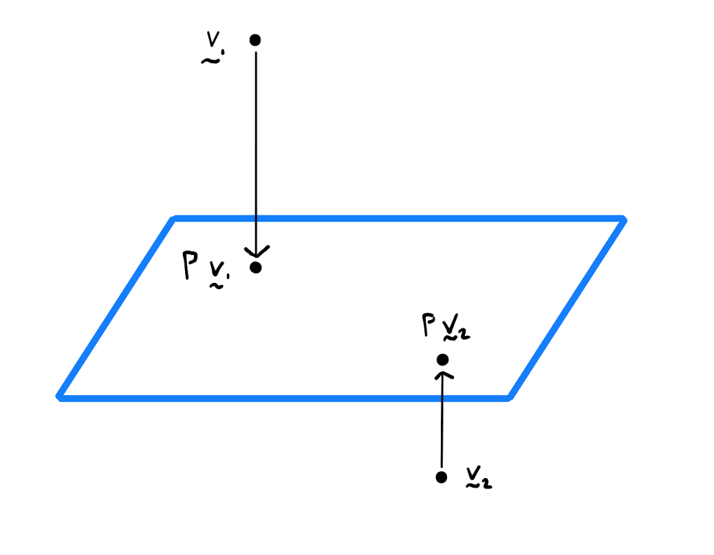
Geometrically a projection maps a vector space onto some linear subspace (typically of lower dimension) and fixes the points of this linear subspace. This is akin to shining a light on an object (the input from the vector space) to cast a shadow on a surface (the output in the image).
Show that \(\mathbf{P} = \begin{pmatrix} \frac{1}{2} & \frac{1}{2} \\ \frac{1}{2} & \frac{1}{2} \end{pmatrix}\) is a projection matrix. Onto what linear subspace does \(\mathbf{P}\) project?
Calculate \[\mathbf{P}^2 = \begin{pmatrix} \frac{1}{2} & \frac{1}{2} \\ \frac{1}{2} & \frac{1}{2} \end{pmatrix} \begin{pmatrix} \frac{1}{2} & \frac{1}{2} \\ \frac{1}{2} & \frac{1}{2} \end{pmatrix} = \begin{pmatrix} \frac{1}{4} + \frac{1}{4} & \frac{1}{4} + \frac{1}{4} \\ \frac{1}{4} + \frac{1}{4} & \frac{1}{4} + \frac{1}{4} \end{pmatrix} = \begin{pmatrix} \frac{1}{2} & \frac{1}{2} \\ \frac{1}{2} & \frac{1}{2} \end{pmatrix} = \mathbf{P}.\] Hence by Definition 1.2.1, \(\mathbf{P}\) is a projection matrix. Now \[\mathbf{P} \begin{pmatrix} x \\ y \end{pmatrix} = \begin{pmatrix} \frac{1}{2} & \frac{1}{2} \\ \frac{1}{2} & \frac{1}{2} \end{pmatrix} \begin{pmatrix} x \\ y \end{pmatrix} = \begin{pmatrix} \frac{x+y}{2} \\ \frac{x+y}{2} \end{pmatrix}.\] Note all points in the image of the map \(\mathbf{P}\) lie on the line \(\left\{ \lambda \begin{pmatrix} 1 \\ 1 \end{pmatrix}: \lambda \in \mathbb{R} \right\}\). Indeed \(\mathbf{P}\) is a projection of \(\mathbb{R}^2\) on this line.
If \(\mathbf{P}\) is a projection matrix then so is \(\mathbf{I}_n - \mathbf{P}\). Furthermore \[\begin{align*} \text{Ker}(\mathbf{I}_n-\mathbf{P}) &= \text{Im} (\mathbf{P}) \\[3pt] \text{Im}(\mathbf{I}_n-\mathbf{P}) &= \text{Ker} (\mathbf{P}) \end{align*}\]
Calculate \[\left( \mathbf{I}_n - \mathbf{P} \right)^2 = \left( \mathbf{I}_n - \mathbf{P} \right)\left( \mathbf{I}_n - \mathbf{P} \right) = \mathbf{I}_n^2 - \mathbf{P} - \mathbf{P} + \mathbf{P}^2 = \mathbf{I}_n - \mathbf{P} - \mathbf{P} + \mathbf{P} = \mathbf{I}_n - \mathbf{P}.\] Therefore \(\mathbf{I}_n - \mathbf{P}\) is a projection matrix.
Let \(\mathbf{x} \in \text{Ker}(\mathbf{P})\), that is, \(\mathbf{Px} = \mathbf{0}\). Then \(\left( \mathbf{I}_n - \mathbf{P} \right) \mathbf{x} = \mathbf{I}_n \mathbf{x} - \mathbf{P} \mathbf{x} = \mathbf{x}\). So \(\mathbf{x} \in \text{Im} \left(\mathbf{I}_n - \mathbf{P}\right)\), and hence \(\text{Ker}(\mathbf{P}) \subseteq \text{Im} \left(\mathbf{I}_n - \mathbf{P}\right)\).
Similarly suppose \(\mathbf{x} \in \text{Im}(\mathbf{P})\), that is, there is some vector \(\mathbf{y}\) such that \(\mathbf{Py} = \mathbf{x}\). It follows that \(\mathbf{Px} = \mathbf{P} (\mathbf{Py}) = \mathbf{P}^2 \mathbf{y} = \mathbf{Py} = \mathbf{x}\), and so \(\left( \mathbf{I}_n - \mathbf{P} \right) \mathbf{x} = \mathbf{x} - \mathbf{Px} =\mathbf{x} - \mathbf{x} = \mathbf{0}\). Therefore \(\mathbf{x} \in \text{Ker} \left(\mathbf{I}_n - \mathbf{P}\right)\), and hence \(\text{Im}(\mathbf{P}) \subseteq \text{Ker} \left(\mathbf{I}_n - \mathbf{P}\right)\).
The result follows from these two inclusions by a simple linear algebra argument regarding dimension.
All eigenvalues of a projection matrix \(\mathbf{P}\) are either \(0\) or \(1\).
Let \(\lambda, \mathbf{v}\) be a eigenvalue, eigenvector pair for \(\mathbf{P}\), that is, \(\mathbf{Px} = \lambda \mathbf{v}\). Then \[\lambda \mathbf{v} = \mathbf{Pv} = \mathbf{P}^2\mathbf{v} = \mathbf{P} \left( \mathbf{Pv} \right) = \mathbf{P} \left( \lambda \mathbf{v} \right) = \lambda \left( \mathbf{P} \mathbf{v} \right) = \lambda^2 \mathbf{v}.\] Therefore \(\lambda^2 = \lambda\). The only two solutions to this equation are \(0\) and \(1\).
Projection matrices are the tool one uses to lower the dimension of a dataset in principal component analysis. The following lemma will play an important role.
Let \(\mathbf{U}\) be a \(p\times r\) matrix whose columns are orthornormal. Then \(\mathbf{P} = \mathbf{UU}^T\) is a projection matrix which sends a vector \(\mathbf{x}\) onto the subspace spanned by the columns of \(\mathbf{U}\).
1.3 Spectral Decomposition
In linear algebra, spectral decomposition is the factorisation of a symmetric matrix into a canonical form described by its eigenvalues and eigenvectors. The spectral decomposition theorem relies on the fact that eigenvectors of a symmetric matrix \(\mathbf{A}\) can be chosen to be mutually orthonormal. This is implied by the following lemma:
Let \(\mathbf{A}\) be an \((n \times n)\)-matrix which is symmetric. Then without loss of generality one can assume that the eigenvectors \(\mathbf{v}_1, \ldots, \mathbf{v}_n\) of \(\mathbf{A}\) are mutually orthogonal.
Consider any two eigenvalue, eigenvector pairs \((\lambda_1, \mathbf{v}_1)\) and \((\lambda_2, \mathbf{v}_2)\) of \(\mathbf{A}\). Calculate that \[ \left( \mathbf{A} \mathbf{v}_1 \right) \cdot \mathbf{v}_2 = \left( \lambda_1 \mathbf{v}_1 \right) \cdot \mathbf{v}_2 = \lambda_1 \mathbf{v}_1 \cdot \mathbf{v}_2\] and \[ \left( \mathbf{A} \mathbf{v}_2 \right) \cdot \mathbf{v}_1 = \left( \lambda_2 \mathbf{v}_2 \right) \cdot \mathbf{v}_1 = \lambda_2 \mathbf{v}_2 \cdot \mathbf{v}_1 = \lambda_2 \mathbf{v}_1 \cdot \mathbf{v}_2.\]
Now since \(\mathbf{A}\) is symmetric, that is \(\mathbf{A} = \mathbf{A}^T\), one has \[\left( \mathbf{A} \mathbf{v}_1 \right) \cdot \mathbf{v}_2 = \mathbf{v}_1 \cdot \left( A^T \mathbf{v}_2 \right) = \mathbf{v}_1 \cdot \left( A \mathbf{v}_2 \right) = \left( \mathbf{A} \mathbf{v}_2 \right) \cdot \mathbf{v}_1.\] Therefore \(\lambda_1 \mathbf{v}_1 \cdot \mathbf{v}_2 = \lambda_2 \mathbf{v}_1 \cdot \mathbf{v}_2\). If \(\lambda_1 \neq \lambda_2\), then necessarily \(\mathbf{v}_1 \cdot \mathbf{v}_2=0\) and the eigenvectors are orthogonal. Alternatively if \(\lambda_1 = \lambda_2\), then \(\mathbf{v}_1\) and \(\mathbf{v}_2\) belong to the same eigenspace and can be chosen to be orthogonal using the Gram-Schmidt algorithm.
Note that for any square matrix one can take eigenvectors of unit length, and hence the required assumption of orthonormality of the eigenvectors of a symmetric matrix \(\mathbf{A}\) follows from Lemma 1.4.1.
Any \(n \times n\) symmetric matrix \(\mathbf{A}\) can be written as \[\mathbf{A} = \mathbf{V} \mathbf{\Lambda} \mathbf{V}^T = \sum\limits_{i=1}^n \lambda_i \mathbf{v}_i \mathbf{v}_i^T\] where
\(\mathbf{\Lambda} = \text{diag} \left( \lambda_1, \cdots, \lambda_n \right)\) is an \(n \times n\) diagonal matrix whose entries are eigenvalues of \(A\);
\(\mathbf{V}\) is an orthogonal matrix whose columns are unit eigenvectors \(\mathbf{v}_1, \ldots, \mathbf{v}_n\) of \(\mathbf{A}\).
Note we can assume in Theorem 1.4.2 and for the remainder of the chapter that \(\lambda_1 \geq \lambda_2 \geq \ldots \geq \lambda_p\). It is also implicit that the ordering of \(\lambda_1, \cdots, \lambda_n\) and \(\mathbf{q}_1, \ldots, \mathbf{q}_n\) is such that \(\lambda_i, \mathbf{q}_i\) form an eigenvalue, eigenvector pair for each \(i\).
Calculate the spectral decomposition of \(\mathbf{A} = \begin{pmatrix} 2 & 3 \\ 3 & 2 \end{pmatrix}\).
Calculate
\[\begin{align*}
\det \left( \mathbf{A} - \lambda \mathbf{I} \right) &= \det \begin{pmatrix} 2-\lambda & 3 \\ 3 & 2-\lambda \end{pmatrix} \\[3pt]
&= (2-\lambda) (2-\lambda) - 9 \\[3pt]
&= \lambda^2 -4\lambda -5 \\[3pt]
&= (\lambda+1) (\lambda-5)
\end{align*}\]
So the eigenvalues of \(\mathbf{A}\) are \(\lambda_1 =-1\) and \(\lambda_2 = 5\).
The eigenvector \(\mathbf{v}_1 = \begin{pmatrix} a \\ b \end{pmatrix}\) satisfies \[\begin{align*} \begin{pmatrix} 3 & 3 \\ 3 & 3 \end{pmatrix} \begin{pmatrix} a \\ b \end{pmatrix} &= \begin{pmatrix} 0 \\ 0 \end{pmatrix} \\[9pt] \iff \qquad \begin{pmatrix} 3a+3b \\ 3a+3b \end{pmatrix} &= \begin{pmatrix} 0 \\ 0 \end{pmatrix} \\[9pt] \iff \qquad \qquad a+b &= 0. \end{align*}\] So take \(\mathbf{v}_1 = \begin{pmatrix} \frac{1}{\sqrt{2}} \\ -\frac{1}{\sqrt{2}} \end{pmatrix}\).
Similarly the eigenvector \(\mathbf{v}_2 = \begin{pmatrix} a \\ b \end{pmatrix}\) satisfies \[\begin{align*} \begin{pmatrix} -3 & 3 \\ 3 & 3 \end{pmatrix} \begin{pmatrix} a \\ b \end{pmatrix} &= \begin{pmatrix} 0 \\ 0 \end{pmatrix} \\[9pt] \iff \qquad \begin{pmatrix} 3b-3a \\ 3a-3b \end{pmatrix} &= \begin{pmatrix} 0 \\ 0 \end{pmatrix} \\[9pt] \iff \qquad \qquad a-b &= 0. \end{align*}\] So take \(\mathbf{v}_2 = \begin{pmatrix} \frac{1}{\sqrt{2}} \\ \frac{1}{\sqrt{2}} \end{pmatrix}\).
Note \(\lvert \mathbf{v}_1 \rvert = \lvert \mathbf{v}_2 \rvert =1\) and the eigenvectors are orthogonal, so the eigenvectors are orthornormal. The Spectral Decomposition theorem tells us that \[\begin{pmatrix} 2 & 3 \\ 3 & 2 \end{pmatrix} = \begin{pmatrix} \frac{1}{\sqrt{2}} & \frac{1}{\sqrt{2}} \\ -\frac{1}{\sqrt{2}} & \frac{1}{\sqrt{2}} \end{pmatrix} \begin{pmatrix} -1 & 0 \\ 0 & 5 \end{pmatrix} \begin{pmatrix} \frac{1}{\sqrt{2}} & -\frac{1}{\sqrt{2}} \\ \frac{1}{\sqrt{2}} & \frac{1}{\sqrt{2}} \end{pmatrix}\] It is easy to verify that this identity holds.It is easy to calculate spectral decompositions using R.
Calculate the spectral decomposition of \(\mathbf{A} = \begin{pmatrix} 4 & 1 & -1 \\ 1 & 3 & 1 \\ -1 & 1 & 2 \end{pmatrix}\) using R.
The following code calculates the eigenvalues and eigenvectors of the matrix:
## eigen() decomposition
## $values
## [1] 4.6751309 3.5391889 0.7856803
##
## $vectors
##            [,1]       [,2]       [,3]
## [1,]  0.8876503 -0.2331920  0.3971125
## [2,]  0.4271323  0.7392387 -0.5206574
## [3,] -0.1721479  0.6317813  0.7557893
One can see that the three eigenvalues are \(4.6751, 3.5392, 0.7857\) with corresponding eigenvectors are \(\begin{pmatrix} 0.8877 \\ 0.4271 \\ -0.1721 \end{pmatrix}, \begin{pmatrix} -0.2332 \\ 0.7392 \\ 0.6318 \end{pmatrix}, \begin{pmatrix} 0.3971 \\ -0.5207 \\ 0.7558 \end{pmatrix}\) respectively. Note the eigenvectors are already presented in a matrix as required. The eigenvalues can placed into a diagonal matrix as required using the following code:
##          [,1]     [,2]      [,3]
## [1,] 4.675131 0.000000 0.0000000
## [2,] 0.000000 3.539189 0.0000000
## [3,] 0.000000 0.000000 0.7856803
The spectral decomposition theorem can be verified by the following code:
##      [,1] [,2] [,3]
## [1,]    4    1   -1
## [2,]    1    3    1
## [3,]   -1    1    2
1.4 Principal Components and Proportion of Variability
As mentioned at the beginning of the chapter, the purpose of principal component analysis is to reduce the dimensionality of a dataset \(X\) by projecting onto a subspace in such a way as to minimise the amount of information lost about the data. Equivalently such a projection should be chosen to maximise the variability of the projected data. Recall that \(\mathbf{X}\) is assumed to be centered.
How a choice of projection can affect variability is illustrated below:
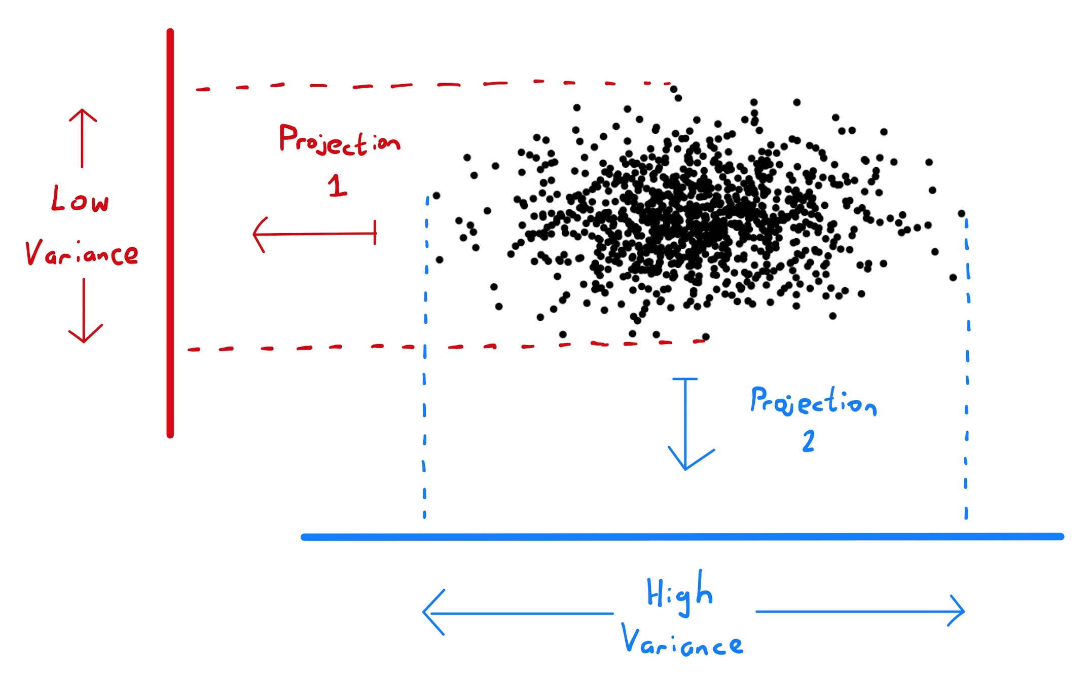
Consider an \(p \times 1\) column vector denoted by \(\mathbf{u}\) of unit length. By Lemma 1.2.3, \(\mathbf{u u}^T\) is a \(p \times p\) matrix that projects a point \(\mathbf{x}\) in \(\mathbb{R}^p\) onto a point \(\tilde{\mathbf{x}}\) on the line spanned by \(\mathbf{u}\). In particular \(\tilde{\mathbf{x}} = \mu \mathbf{u}\) where \(\mu\) is the constant \(\mathbf{u}^T \mathbf{x}\).
The choice of \(\mathbf{u}\) that maximises the variability of datapoints in \(\mathbf{X}\) under projection by \(\mathbf{u u}^T\) is the unit eigenvector \(\mathbf{v}_1\) of the sample covariance matrix \(\mathbf{S} = \frac{1}{n} \mathbf{X}^T \mathbf{X}\) that corresponds to the largest eigenvalue.
Recall \(\mathbf{X} = \begin{pmatrix} \mathbf{x}^T_1 \\ \mathbf{x}^T_2 \\ \vdots \\ \mathbf{x}^T_n \end{pmatrix}\). In order for the datapoints to be aligned as column vectors under the projection, one must calculate \(\mathbf{u u}^T \mathbf{X}\). The \(i^{th}\) row of \(\mathbf{u u}^T \mathbf{X}\) will be \(\tilde{\mathbf{x}}_i = \mathbf{u u}^T \mathbf{x}_i = \mu_i \mathbf{u}\) where \(\mu_i=\mathbf{u}^T\mathbf{x}\). Our motivation for principal component analysis dictates that one should maximise the variance of the \(\tilde{\mathbf{x}}_i\). Note that \[\text{arg max}_{\mathbf{u}} \text{Var} \left( \tilde{\mathbf{x}}_1, \ldots, \tilde{\mathbf{x}}_n \right) = \text{arg max}_{\mathbf{u}} \text{Var} \left( \mu_1, \ldots, \mu_n \right)\] Now \[\begin{align*} \text{Var} \left( \mu_1, \ldots, \mu_n \right) &= \frac{1}{n} \sum\limits_{i=1}^n \mu_i^2 \\[3pt] &= \frac{1}{n} \sum\limits_{i=1}^n \left( \mathbf{u}^T\mathbf{x}_i \right)^2 \\[3pt] &= \frac{1}{n} \sum\limits_{i=1}^n \mathbf{u}^T \mathbf{x}_i \mathbf{x}_i^T \mathbf{u} \\[3pt] &= \frac{1}{n} \mathbf{u}^T \left( \sum\limits_{i=1}^n \mathbf{x}_i \mathbf{x}_i^T \right) \mathbf{u} \\[3pt] &= \frac{1}{n} \mathbf{u}^T \mathbf{X}^T \mathbf{X} \mathbf{u} \\[3pt] &= \mathbf{u}^T \mathbf{S} \mathbf{u} \end{align*}\] where the first equality has used that the data is centered, the penultimate equality has used Lemma 1.1.3, and \(\mathbf{S}\) is the sample covariance matrix. Using previously established notation, let \(\lambda_1 \geq \lambda_2 \geq \cdots \geq \lambda_p\) be the eigenvalues of \(\mathbf{S}\), and \(\mathbf{v}_1, \mathbf{v}_2, \ldots, \mathbf{v}_p\) be the corresponding eigenvectors. Now applying the Spectral Decomposition Theorem obtain \[\begin{align*} \mathbf{u}^T \mathbf{S} \mathbf{u} &= \mathbf{u}^T \left( \sum\limits_{i=1}^p \lambda_i \mathbf{v}_i \mathbf{v}_i^T \right) \mathbf{u} \\[3pt] &= \sum\limits_{i=1}^p \lambda_i \left( \mathbf{u}^T \mathbf{v}_i \right)^2 \\[3pt] &\leq \sum\limits_{i=1}^p \lambda_i \left( \mathbf{u}^T \mathbf{v}_i \right)^2 \\[3pt] &= \lambda_1. \end{align*}\]
So \(\text{Var} \left( \mu_1, \ldots, \mu_n \right)\) is bounded above by \(\lambda_1\). However more importantly, one can observe from the inequality that this bound is achieved when \(\mathbf{u} = \mathbf{v}_1\).
Motivated by the previous lemma is the following definition:
The vector \(\mathbf{v}_1\) of \(\mathbf{X}\) is known as the first principal component of \(\mathbf{X}\).
The first principal component represents the direction in \(\mathbb{R}^p\) in which the data are most variable.
This theory easily extends to the case of a higher dimensional subspace on which we want to project. The second principal component is the direction orthogonal to \(\mathbf{v}_1\) of next most variability. A proof similar to that of Lemma 1.4.2 shows that the second principal component is the eigenvector \(\mathbf{v}_2\) of \(\mathbf{S}\) corresponding to the second largest eigenvalue.
The \(i^{th}\) principal component is the direction orthogonal to \(\mathbf{v}_1, \mathbf{v}_2, \ldots, \mathbf{v}_{i-1}\) of most variability, and is given by the eigenvector \(\mathbf{v}_i\) of \(\mathbf{S}\) corresponding to the \(i^{th}\) largest eigenvalue.
From the proof of Lemma 1.4.2, one knows that the variance in the direction of the first principal component is \(\lambda_1\). This leads to the following definition.
The proportion of variability explained by the first principal component is \(\frac{\lambda_1}{\lambda_1 + \ldots + \lambda_p}\).
Indeed the definition, like above, generalises to the case of the subspace onto which projection occurs is of dimension greater than \(1\).
The proportion of variability explained by the first \(r\) principal components is \(\frac{\lambda_1 + \ldots + \lambda_r}{\lambda_1 + \ldots + \lambda_p}\).
A line plot of the proportion of variability explained by the \(k^{th}\) principal component against \(k\) is known as a scree plot.
Download the file Country-data.csv from the Moodle page. The data details a number of socio-economic and health measures for a number of countries. Use R to calculate the first two principal components of the data, plot these components against each other and state the proportion of the variance explained by these two principal components.
Begin by loading the data into R:
##               country child_mort exports health imports income inflation
## 1         Afghanistan       90.2    10.0   7.58    44.9   1610      9.44
## 2             Albania       16.6    28.0   6.55    48.6   9930      4.49
## 3             Algeria       27.3    38.4   4.17    31.4  12900     16.10
## 4              Angola      119.0    62.3   2.85    42.9   5900     22.40
## 5 Antigua and Barbuda       10.3    45.5   6.03    58.9  19100      1.44
## 6           Argentina       14.5    18.9   8.10    16.0  18700     20.90
##   life_expec total_fer  gdpp
## 1       56.2      5.82   553
## 2       76.3      1.65  4090
## 3       76.5      2.89  4460
## 4       60.1      6.16  3530
## 5       76.8      2.13 12200
## 6       75.8      2.37 10300
Note the first column of the dataframe is the name of the countries. This is not a numerical value and will not contribute to principal component analysis. Hence we drop this column from the dataframe.
The function prcomp() performs principal component analysis. The scale parameter of prcomb() indicates whether the data should be scaled so that every variable has variance \(1\). By default the scale parameter is FALSE, however scaling can often lead to improved performance. The principal components, that is the directions in which to project, can be accessed in the value rotation of prcomp(). By restricting to the first two columns, one can obtain the required principal components.
##                   PC1          PC2
## child_mort -0.4195194 -0.192883937
## exports     0.2838970 -0.613163494
## health      0.1508378  0.243086779
## imports     0.1614824 -0.671820644
## income      0.3984411 -0.022535530
## inflation  -0.1931729  0.008404473
## life_expec  0.4258394  0.222706743
## total_fer  -0.4037290 -0.155233106
## gdpp        0.3926448  0.046022396
The value x of prcomp() applies the projection matrix of the eigenvectors to the data. By restricting the output to the first two columns, one can obtain the coordinates of the data projected onto the first two principal components. This is the data to be plotted.
print(head(results$x[,1:2]))
plot(results$x[,1],results$x[,2],
     main="Principal Components of Socio-economic and Health Country Data",
     xlab="PCA1",
     ylab="PCA2",
     cex=0.5,
     pch=19)
The value \(\textit{sdev}\) gives a vector of the square root of the eigenvalues, which is equivalently the standard deviation of the projection of the data in the direction \(\mathbf{v}_i\). By summing the square of the first two entries and dividing by the sum of the square of the entries gives the proportion of the variability explained by the first \(2\) principal components.
## [1] 0.6313337If the variables described by data have vastly different magnitudes, then PCA may perform poorly. This effect is caused by the fact the relatively large scale variables will most likely have significantly larger variance. Since PCA is an exercise in maximising variance, in this scenario PCA may indicate that one should simply disregard the other relatively smaller variables. All insight from these other variables is lost. To avoid this loss of information, one should simply normalise all variables to have a standard deviation of \(1\).