Chapter 12 Logistic Regression
12.1 Motivation
In previous weeks, we have been focusing on regression problems, where the response variables are quantitative. Here we will see how we can work with qualitative response variables which leads to classification problems.
Qualitative variables take values in an unordered set. For example:
patient status \(\in\) \(\{\)dead, alive\(\}\)
weather \(\in\) \(\{\) rainy, cloudy, sunny \(\}\)
Take the case where we are trying to predict a patient’s outcome. We might have access to a number of variables (quantitative or qualitative) that indicate the patient’s health status, e.g. height, weight, age, gender, heart rate, consciousness.
Quantitative variables: height, weight, age, heart rate
Qualitative variables: gender, consciousness
The task here is to build a function that takes features \(X\) (e.g. height, age) as input and predicts the value for the response \(Y\) (i.e. dead or alive). While predicting the response itself is valuable, we often want to estimate the probability that \(X\) maps to one of the potential categories.
For example, if we are looking at insurance fraud, estimating the probability that a claim is fraudulent is often more valuable to a bank than the actual classification of the event in fraudulent or not. The same applies if we are looking at health outcomes, say for example, whether someone is likely to have cancer or not in the future. While life threatening, estimating probabilities and consequently the risk associated to a patient (ideally over time) is more valuable than asserting their future state.
Example: The Default data set
Here we will look at the Default dataset that contains information on credit card balance and income for 10,000 people, and also whether they have defaulted and whether they are a student or not.
library("ISLR2")##
## Attaching package: 'ISLR2'## The following object is masked _by_ '.GlobalEnv':
##
## Hitters## The following object is masked from 'package:MASS':
##
## Boston## The following objects are masked from 'package:ISLR':
##
## Auto, Creditdata(Default)
head(Default)## default student balance income
## 1 No No 729.5265 44361.625
## 2 No Yes 817.1804 12106.135
## 3 No No 1073.5492 31767.139
## 4 No No 529.2506 35704.494
## 5 No No 785.6559 38463.496
## 6 No Yes 919.5885 7491.559It’s good practice to check for missing data, here we check for missing values in the default variable:
print(paste("Missing data:", sum(is.na(Default$default)),sep=" ",collapse=""))## [1] "Missing data: 0"table(Default$default,dnn="Default")## Default
## No Yes
## 9667 333We now produce a pairs plot to look at the relationship between all variables in our dataset:
pairs(Default)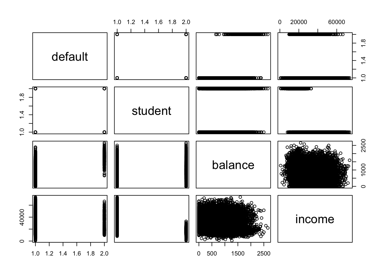 The
The pairs plot isn’t particularly interesting but we note that balance and income are the only two quantitative predictors. Let’s produce a scatter of balance vs income and colour the points by the default variable.
library(scales) #loads the alpha function to add transparency to coloursplot(Default$balance, Default$income, col=alpha(c("red","blue")[Default$default],0.6), pch=3, xlab="Balance", ylab="Income")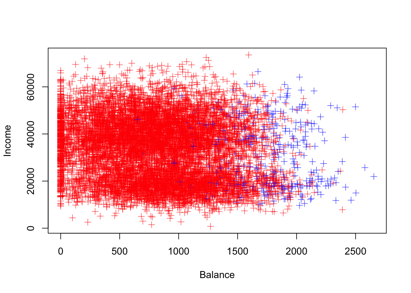
There seems to be a pattern emerging where users with a high balance are more likely to default. Let’s inspect this using a boxplot:
boxplot(balance~default, data=Default)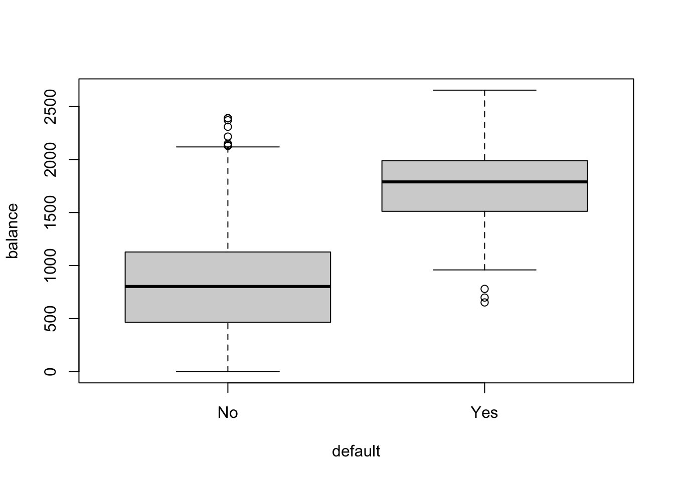
boxplot(income~default,data=Default)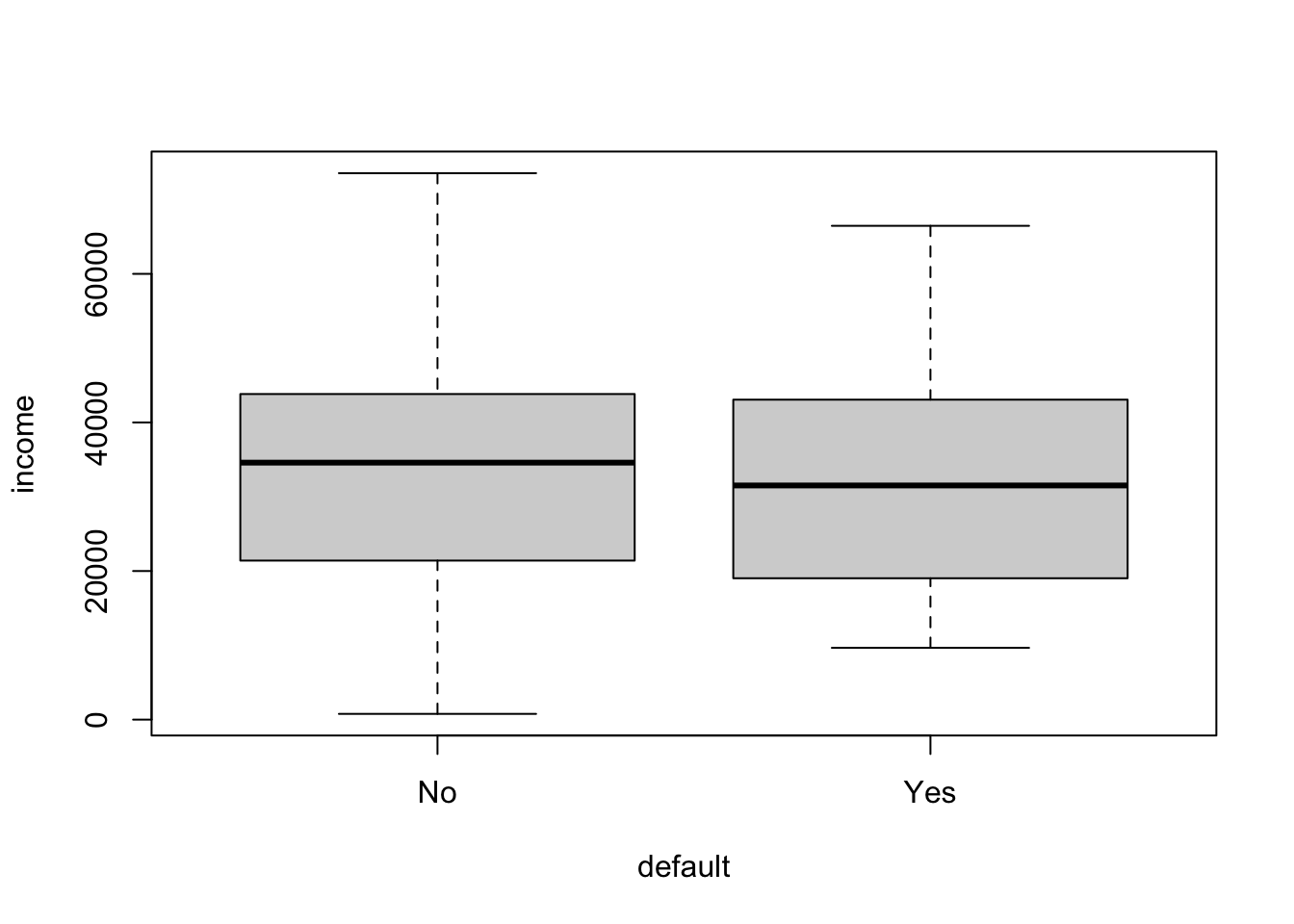
It seems that balance is likely to be a good predictor for whether someone is likely to default or not, but not income.
Let’s take default as our response variable Y and we will rewrite it as:
\[ Y = \begin{cases} 0, \; if \;\; No,\\ 1, \; if \;\; Yes. \end{cases} \]
Note that by treating the response \(Y\) as a quantitative variable, we can apply the linear regression model (\(E(Y|X=x)=\beta_0+\beta_1x\)):
lm.fit = lm(as.numeric(default == "Yes") ~ balance, data=Default)
summary(lm.fit)
##
## Call:
## lm(formula = as.numeric(default == "Yes") ~ balance, data = Default)
##
## Residuals:
## Min 1Q Median 3Q Max
## -0.23533 -0.06939 -0.02628 0.02004 0.99046
##
## Coefficients:
## Estimate Std. Error t value Pr(>|t|)
## (Intercept) -0.075191959 0.003354360 -22.42 <0.0000000000000002 ***
## balance 0.000129872 0.000003475 37.37 <0.0000000000000002 ***
## ---
## Signif. codes: 0 '***' 0.001 '**' 0.01 '*' 0.05 '.' 0.1 ' ' 1
##
## Residual standard error: 0.1681 on 9998 degrees of freedom
## Multiple R-squared: 0.1226, Adjusted R-squared: 0.1225
## F-statistic: 1397 on 1 and 9998 DF, p-value: < 0.00000000000000022Let’s explore it further by producing a scatter plot of balance vs default and add the regression line to the plot.
plot(Default$balance, as.numeric(Default$default=="Yes"),col="red",xlab="balance",ylab="default")
abline(lm.fit, col="blue", lwd = 2)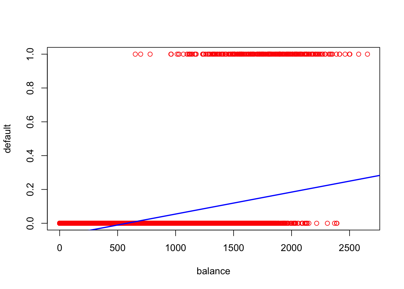
par(mfrow=c(1,2))
plot(y=resid(lm.fit), x=fitted(lm.fit))
qqnorm(resid(lm.fit))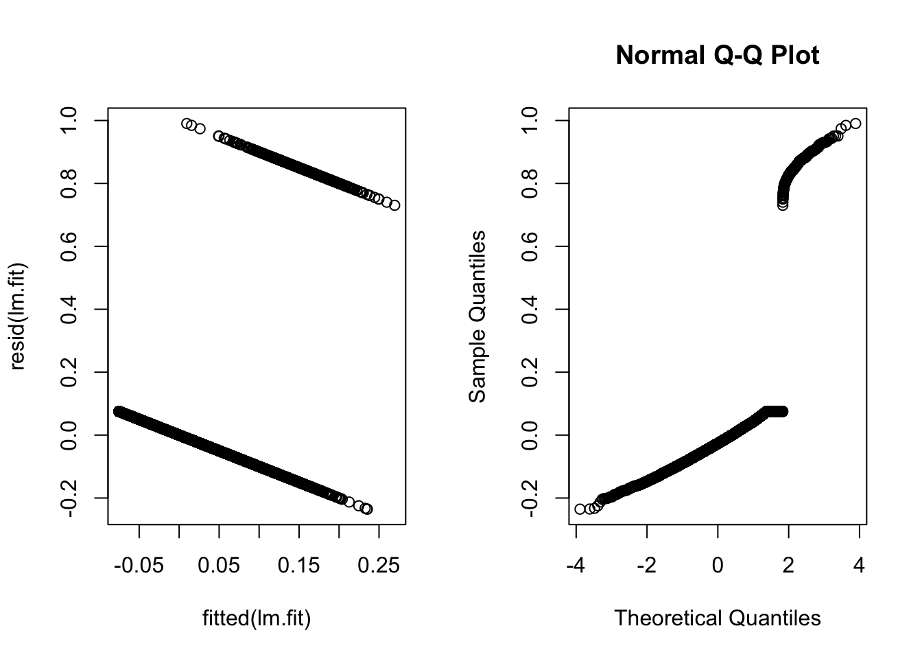
par(mfrow=c(1,1))This doesn’t seem like a particularly good model…
12.2 Simple Logistic Regression
Note that in the Default data example, \(E(Y|X=x)=P(Y=1|X=x)\), which means the linear regression model is trying to predict the probability of defaulting. Unfortunately, for balances close to zero we predict a negative probability of defaulting; if we were to predict for very large balances, we would get values bigger than 1. These predictions are not sensible, since of course the true probability of defaulting, regardless of credit card balance, must fall between 0 and 1.
To avoid the inadequacies of the linear model fit on a binary response, we must model the probability of our response using a function that gives outputs between 0 and 1 for all values of \(X\). In logistic regression, we use the logistic function to transform/map the outputs to \((0,1)\).
Say \(p(X)=P(Y=1|X)\), we write the logistic function \[ p(X)=\frac{\exp(\beta_0+\beta_1X)}{1+\exp(\beta_0+\beta_1X)} \] This transformation would guarantee that \(p(X)∈(0,1)\) for any \(\beta_0\), \(\beta_1\), and \(X\). Note that \[ \ln\frac{p(X)}{1−p(X)}=\beta_0+\beta_1X \] and we can modify this to take any number of response variables. This transformation is called the logit transformation.
The standard approach for producing estimates \(\beta_0\) and \(\beta_1\) of the regression coefficients in the logistic regression model is to use maximum likelihood estimation. One of the advantages of this method is that maximum likelihood estimators have a number of nice theoretical properties which can be exploited to derive confidence intervals for the regression coefficients, perform hypothesis tests, and so on. In R, all this goes on under the hood when we use the glm function to fit the logistic regression model. When using the glm function, we need to set the argument family="binomial" to indicate that we want to fit a logistic regression model, and not some other kind of generalised linear model.
Now let’s try to fit a linear logistic regression model to the Default dataset using the glm function in R with family set to binomial.
glm.fit = glm(as.numeric(Default$default=="Yes") ~ balance, data = Default, family = "binomial")
summary(glm.fit)
##
## Call:
## glm(formula = as.numeric(Default$default == "Yes") ~ balance,
## family = "binomial", data = Default)
##
## Deviance Residuals:
## Min 1Q Median 3Q Max
## -2.2697 -0.1465 -0.0589 -0.0221 3.7589
##
## Coefficients:
## Estimate Std. Error z value Pr(>|z|)
## (Intercept) -10.6513306 0.3611574 -29.49 <0.0000000000000002 ***
## balance 0.0054989 0.0002204 24.95 <0.0000000000000002 ***
## ---
## Signif. codes: 0 '***' 0.001 '**' 0.01 '*' 0.05 '.' 0.1 ' ' 1
##
## (Dispersion parameter for binomial family taken to be 1)
##
## Null deviance: 2920.6 on 9999 degrees of freedom
## Residual deviance: 1596.5 on 9998 degrees of freedom
## AIC: 1600.5
##
## Number of Fisher Scoring iterations: 8First note that now the fitted values in our regression are between \(0\) and \(1\).
summary(glm.fit$fitted.values)## Min. 1st Qu. Median Mean 3rd Qu. Max.
## 0.0000237 0.0003346 0.0021888 0.0333000 0.0142324 0.9810081And a plot of our model output looks far more sensible. In the plot below, we have the raw data in red, the fitted logistic curve in blue, and the fitted values in black.
plot(Default$balance, as.numeric(Default$default=="Yes"),col="red",xlab="balance",ylab="default")
points(glm.fit$data$balance,glm.fit$fitted.values, col = "black", pch = 4)
curve(predict(glm.fit,data.frame(balance = x),type="resp"),col="blue",lwd=2,add=TRUE)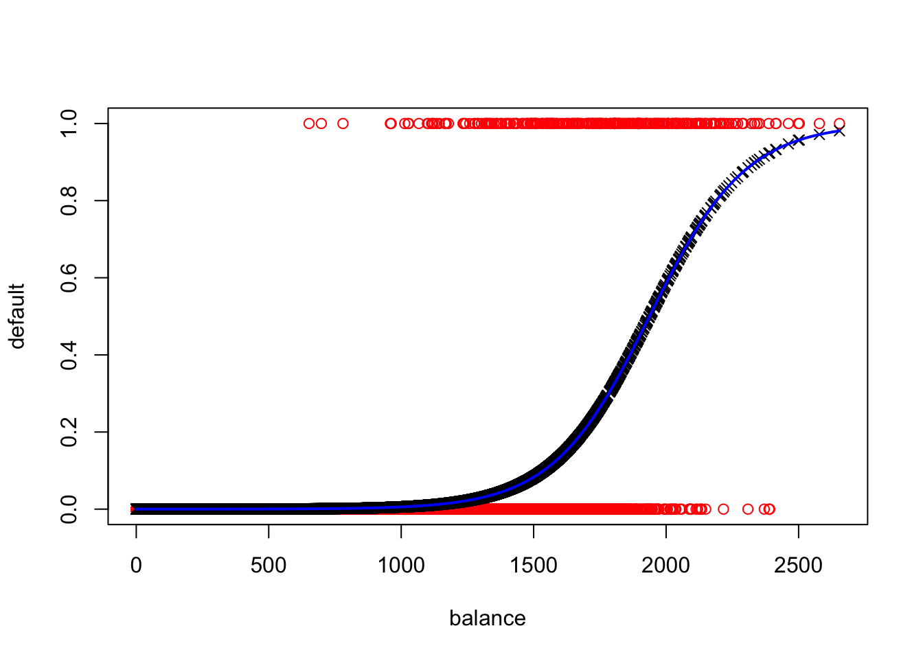
From the logistic regression summary, we have estimates for \(\beta_0\) and \(\beta_1\) and we can estimate the probability of default for an individual given their balance. Say someone has a balance of \(£500\), then
\[ \hat{p}(X)=\frac{\exp(\hat{\beta_0}+\hat{\beta_1}X)}{1+\exp(\hat{\beta_0}+\hat{\beta_1}X)} \] and \(\hat{p}\) equals
exp(sum(glm.fit$coefficients*c(1,500)))/(1+exp(sum(glm.fit$coefficients*c(1,500))))## [1] 0.0003699132Repeat the above experiment with different values for the balance variable. What do you see?
12.3 Logistic regression with several variables
We can extend the logit transformation to accommodate any number of response variables. Simply write:
\[ \ln\frac{p(X)}{1−p(X)}=\beta_0+\beta_1X_1+\beta_2X_2+…+\beta_pX_p \] and \[ p(X)=\frac{\exp(\beta_0+\beta_1X_1+\beta_2X_2+…+\beta_pX_p)}{1+\exp(\beta_0+\beta_1X_1+\beta_2X_2+…+\beta_pX_p)} \]
And this can even be extended to the Generalised Additive Models to allow for non-linear relationships to be considered in the model by: \[ \ln\frac{p(X)}{1−p(X)}=\beta_0+f_1(X_1)+f_2(X_2)+…+f_p(X_p) \]
12.4 Interpreting coefficients
The interpretation of the coefficients in the logistic regression isn’t as simple as in the linear regression scenario since we are predicting the probability of an outcome rather than the outcome itself.
If \(\beta_1=0\), then there is no relationship between \(Y\) and \(X\). If \(β_1>0\), \(X\) gets larger and so does the probability that \(Y=1\). If \(\beta_1<0\), the opposite happens, that is, as \(X\) gets larger, the probability that \(Y=1\) gets smaller.
12.5 Significance
We also want to investigate whether the coefficient values are significant. That is, we want to know whether the coefficients are statistically different from zero.
In linear regression, we use a \(t\)-test to check significance for coefficients. In logistic regression, we use a \(z\)-test (normal test) instead. Let’s look at the summary of the regression:
summary(glm.fit) #default vs balance##
## Call:
## glm(formula = as.numeric(Default$default == "Yes") ~ balance,
## family = "binomial", data = Default)
##
## Deviance Residuals:
## Min 1Q Median 3Q Max
## -2.2697 -0.1465 -0.0589 -0.0221 3.7589
##
## Coefficients:
## Estimate Std. Error z value Pr(>|z|)
## (Intercept) -10.6513306 0.3611574 -29.49 <0.0000000000000002 ***
## balance 0.0054989 0.0002204 24.95 <0.0000000000000002 ***
## ---
## Signif. codes: 0 '***' 0.001 '**' 0.01 '*' 0.05 '.' 0.1 ' ' 1
##
## (Dispersion parameter for binomial family taken to be 1)
##
## Null deviance: 2920.6 on 9999 degrees of freedom
## Residual deviance: 1596.5 on 9998 degrees of freedom
## AIC: 1600.5
##
## Number of Fisher Scoring iterations: 8In this case, we see that balance is likely to be a good predictor for default and the \(z\)-test indicates that we should include this variable in our model. And as we had seen before, the higher the balance, the more likely someone is to default.