Analysis

This next section will provide a step-by-step walk through of the methodology conducted for this analysis. The methods used are: - Bi-variate OLS model - Multi-variate OLS model - Spatial Auto-correlation using local Moran’s I - Spatial Lag Model and Spatial Errors Model - Geographically Weighted Regression

Lets load our libraries:

And then read in our data:

Some of the field names in the MSOA shapefile were abbreviated and haven’t been given the most intuitive of names so we need to rename them:

data <- data%>%
  rename(code = MSOA11C,
         totcases = ttl_css,
         p_0_15 = pc_0_15,
         hh_tot = hhlds_t,
         p_hhwdc = pct_hh_,
         p_lphh = pct_lp_,
         p_1phh = pct_1p_,
         pct_oth = pct_thr,
         pct_oo = pct_wnt,
         pct_det = pct_dtc,
         pct_ql4 = pct_q4_,
         mn_hh_i = mn_hh_n,
         pct_obe = pct_16_,
         le_f = le_feml,
         le_m = le_male,
         gs_m2 = gs_r_m2,
         gs_ha = gs_ar_h)

We need to transform the total cases and greenspace area fields to the following:

• pr_cases = proportion of covid-19 cases out of the msoa population (this represents the prevalence)

• pr_gsm2/ha = proportion of proximate public green space area (> 2 hectares with 5 min proximity) to the total land area of each msoa.

data <- data%>%
  mutate(pr_cases = totcases / pop * 100,
         pr_gsm2 = gs_m2 / area_m2 * 100,
         pr_gsha = gs_ha / area_ha * 100)

Exploratory Spatial Data Analysis

Lets do some EDA and see what the distributions are for the proportions of proximate public green space in the London MSOAS and the proportion of total COVID-19 cases to the population of each MSOA.

Looking at the distribution for the proportion of proximate public green space in each MSOA, it can be concluded that it is of a normal distribution.

data%>%
  ggplot(aes(x=pr_gsha)) +
  geom_histogram(position="identity", 
                 alpha=0.5, 
                 bins=15, 
                 fill="lightblue2", col="lightblue3")+
  geom_vline(aes(xintercept=mean(pr_gsha)),
             color="blue",
             linetype="dashed")+
  labs(title="Distribution of the proportion of proximate public green spaces that are 2 hectares or more,
       within a 5 minute walking distance to the total land area of each MSOA.",
       x="Proportion of defined greenspace",
       y="Frequency")+
  theme_classic()+
  theme(plot.title = element_text(hjust = 0.5))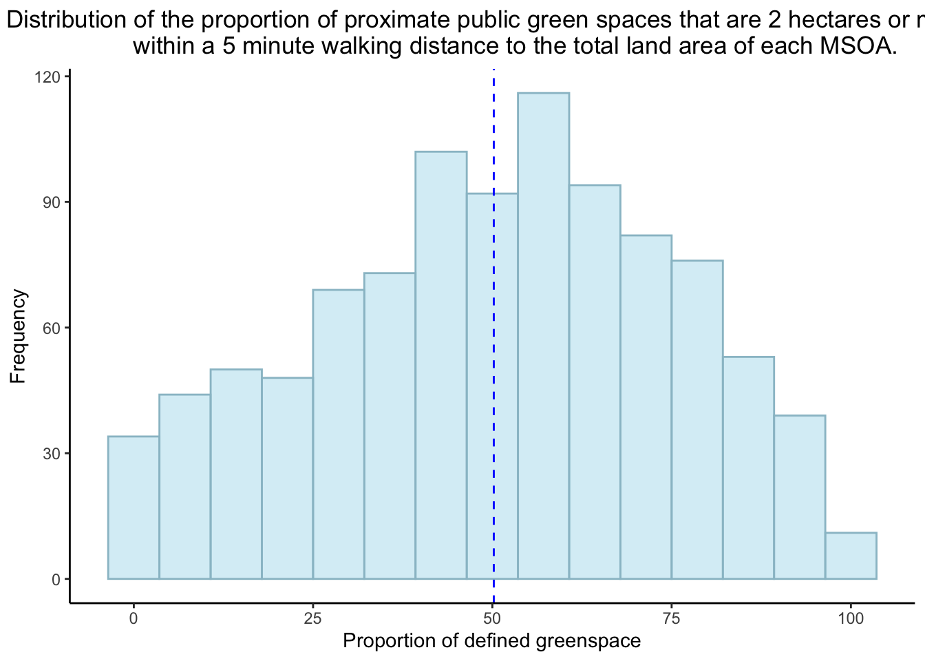

However, the distribution of the proportion of total COVID-19 cases to the population of each MSOA (between 22/09/2020 to 08/12/2020) appears to be positively skewed.

data%>%
  ggplot(aes(x=pr_cases)) +
  geom_histogram(position="identity", 
                 alpha=0.5, 
                 bins=15, 
                 fill="lightblue2", col="lightblue3")+
  geom_vline(aes(xintercept=mean(pr_cases)),
             color="blue",
             linetype="dashed")+
  labs(title="Distribution of the proportion of total COVID-19 cases to the population
       of each MSOA.",
       x="Proportion of COVID-19 cases (%)",
       y="Frequency")+
  theme_classic()+
  theme(plot.title = element_text(hjust = 0.5))

Spatial Autocorrelation

For exploratory purposes we will explore whether spatial autocorrelation is present in the proportion of proximate green space variable. Given the literature that exists, we can be confident that we will find significant results both at global and local levels using Moran’s I, Geary’s C and Getis-Ords statistics.

To begin, we will plot a simple interactive map to visualise the spatial variations in the proportion of proximate public green space for each MSOA. We can see that some clustering exists with both high proportions of proximate public green space and low proportions.

tmap_mode("view")

## tmap mode set to interactive viewing

tm_shape(data) +
  tm_polygons("pr_gsha",
              style="jenks",
              palette="BuGn",
              n=4,
              midpoint=NA,
              popup.vars=c("name", "pr_gsha"),
              title="Proportion of proximate public green space to total land area (%)")

We will run:

• Moran’s I

• Geary’s C

• Getis-Ord

global spatial statistics to quantify our initial observations:

We will then create a neighbours list using Queens Contiguity Neighbours. A snap value argument of 0.0001 was recommended by this article to accurately identify the required neighbours.

msoa_nb <- data%>%
  poly2nb(., queen=T, snap = 0.0001) #snap value needed

Now we can plot the MSOA centroids and Queens contiguity neighbours.

plot(msoa_nb, st_geometry(coordsMSOA), col="red")
plot(data$geometry, add=T)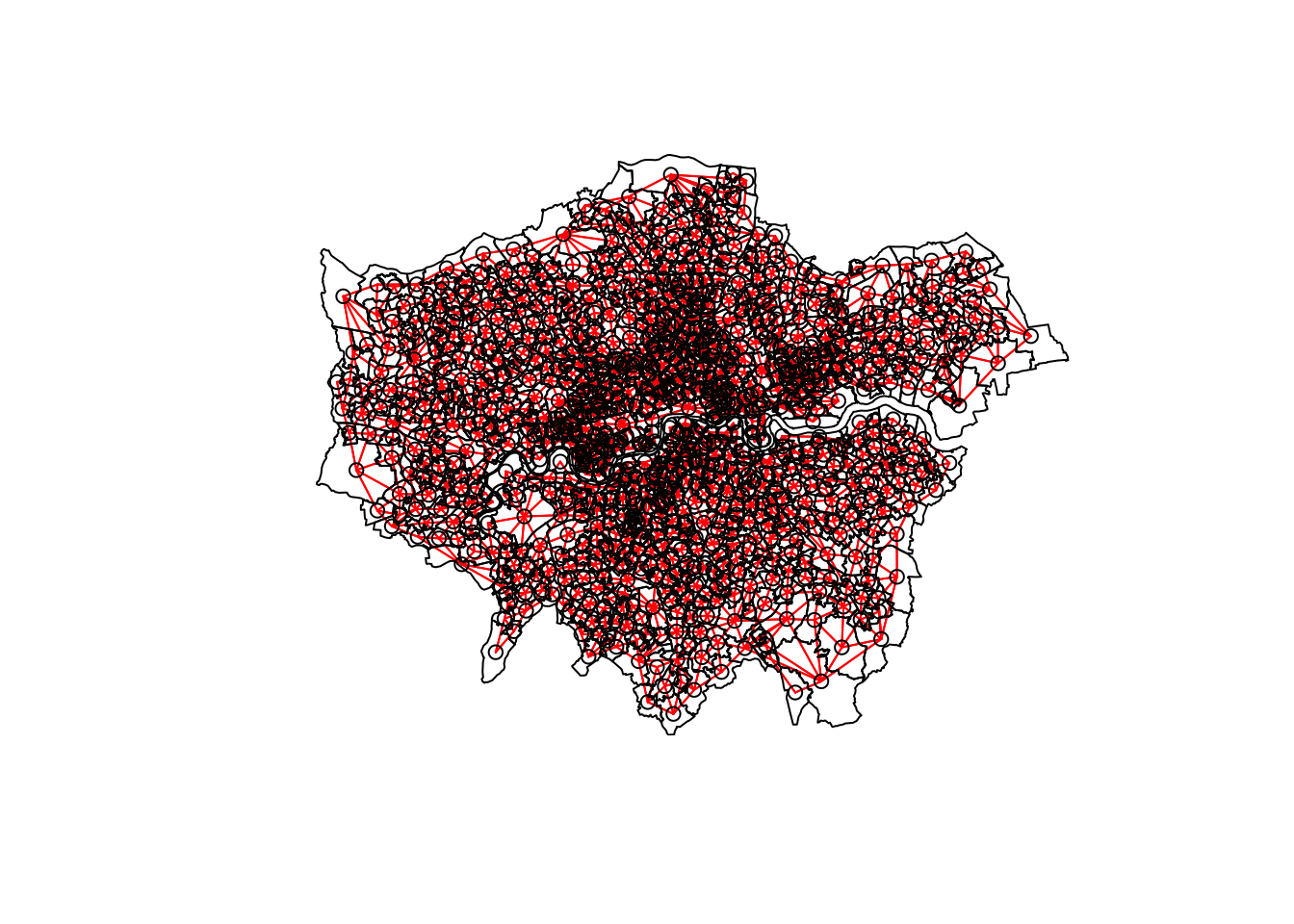

Now we need to create a spatial weights matrix from the MSOA neighbours list:

msoa.lw <- msoa_nb %>%
  nb2listw(., style="C")

We now have the parameters needed to run the Moran’s I, Geary’s C and Getis-Ords global spatial statistics.

Moran’s I - The Moran’s I score shows moderate spatial autocorrelation exists (0.212011)

I_MSOA_Global_prgs <- data%>%
  pull(pr_gsha) %>%
  as.vector()%>%
  moran.test(., msoa.lw)

I_MSOA_Global_prgs

## 
##  Moran I test under randomisation
## 
## data:  .  
## weights: msoa.lw    
## 
## Moran I statistic standard deviate = 11.354, p-value < 2.2e-16
## alternative hypothesis: greater
## sample estimates:
## Moran I statistic       Expectation          Variance 
##      0.2120111379     -0.0010183299      0.0003520366

Geary’s C - The Geary’s C spatial statistic shows us that positive spatial autocorrelation or similar values are clustering because the statistic is less than 1.0 at 0.78959

C_MSOA_Global_prgs <- 
  data %>%
  pull(pr_gsha) %>%
  as.vector()%>%
  geary.test(., msoa.lw)

C_MSOA_Global_prgs

## 
##  Geary C test under randomisation
## 
## data:  . 
## weights: msoa.lw 
## 
## Geary C statistic standard deviate = 10.091, p-value < 2.2e-16
## alternative hypothesis: Expectation greater than statistic
## sample estimates:
## Geary C statistic       Expectation          Variance 
##      0.7895958723      1.0000000000      0.0004347273

Getis-Ord - The Getis-Ord statistic is more than the expected value - This means that high values are clustered spatially

G_MSOA_Global_prgs <- 
  data %>%
  pull(pr_gsha) %>%
  as.vector()%>%
  globalG.test(., msoa.lw)

G_MSOA_Global_prgs

## 
##  Getis-Ord global G statistic
## 
## data:  . 
## weights: msoa.lw 
## 
## standard deviate = 9.1091, p-value < 2.2e-16
## alternative hypothesis: greater
## sample estimates:
## Global G statistic        Expectation           Variance 
##       1.105502e-03       1.018330e-03       9.158069e-11

The spatial statistics that were ran above show us that on a global scale there is spatial clustering/ spatial autocorrelation within the proportion of proximate public green space variable. This was hypothesised when observing the interactive plot of the variable.

Now local spatial statistics will be run to quanitfy the local spatial autocorrelation.

Local Moran’s I

I_MSOA_Local_prgs <- data %>%
  pull(pr_gsha) %>%
  as.vector()%>%
  localmoran(., msoa.lw)%>%
  as_tibble()

slice_head(I_MSOA_Local_prgs, n=5)

## # A tibble: 5 x 5
##   Ii          E.Ii          Var.Ii     Z.Ii        `Pr(z > 0)` 
##   <localmrn>  <localmrn>    <localmrn> <localmrn>  <localmrn>  
## 1  3.96340828 -0.0019495754 0.3294010   6.90907583 2.439106e-12
## 2  0.46176462 -0.0010634047 0.1805973   1.08909069 1.380569e-01
## 3  0.07028047 -0.0012406389 0.2104812   0.15589333 4.380586e-01
## 4  0.82157792 -0.0008861706 0.1506517   2.11899471 1.704546e-02
## 5 -0.02802417 -0.0008861706 0.1506517  -0.06991829 5.278707e-01

#Add local values to new dataframe
data2 <- data%>%
  mutate(prgs_I =as.numeric(I_MSOA_Local_prgs$Ii))%>%
  mutate(prgs_Iz =as.numeric(I_MSOA_Local_prgs$Z.Ii))

Local Getis-Ord

#Local Getis Ord for Hot and Cold spots
Gi_MSOA_Local_prgs <- data%>%
  pull(pr_gsha) %>%
  as.vector()%>%
  localG(., msoa.lw)

head(Gi_MSOA_Local_prgs)

## [1] -3.87971776 -1.02606864 -1.27281870  1.83296359  0.09303408  0.99850185

#Joining
data2 <- data2 %>%
  mutate(prgs_G = as.numeric(Gi_MSOA_Local_prgs))

To understand the results, let’s map them and see what appears significant.

Plot of Local Moran’s I results:

library(RColorBrewer)

breaks1<-c(-1000,-2.58,-1.96,-1.65,1.65,1.96,2.58,1000)
MoranColours<- brewer.pal(8, "PiYG")

tmap_mode("view")

## tmap mode set to interactive viewing

tm_shape(data2) +
  tm_polygons("prgs_Iz",
              style="fixed",
              breaks=breaks1,
              palette=MoranColours,
              midpoint=NA,
              title="Local Moran's I: Results for the Proportion of proximate public green spaces
              across London.")

Plot the Local Getis-Ords statistics to visualise the hot and cold spots:

GIColours<- rev(brewer.pal(8, "RdBu"))

tmap_mode("view")

## tmap mode set to interactive viewing

tm_shape(data2) +
  tm_polygons("prgs_G",
              style="fixed",
              breaks=breaks1,
              palette=GIColours,
              midpoint=NA,
              title="Local Getis-Ord: Proportion of proximate public green spaces across London.")

The two plots show similar spatial clustering however the local Getis Ord’s results illustrate a more distinguishable difference between hot and cold spots of spatial clustering. This distinction can be observed when looking at the areas around Richmond Park and the City of London. Local Getis Ord’s results demonstrate a clearer idea of where high and low values are clustering.

Analysing COVID-19 Prevalence in London MSOAS

This next part of the analysis will be investigating COVID-19 prevalence in London MSOAs. Both global and local models with and without the greenspace variable will be included to observe its role in explaining COVID-19 prevalence.

We will begin by running basic, global Ordinary Least Square (OLS) Models to examine the relationships between COVID-19 and the proportion of proximate public green space and other explanatory variables.

Since the proportion of COVID-19 variable is positively skewed, it will be logged for the following models. This is a quick plot of its distribution after it has had a log-normal transformation.

The first OLS model will be a bi-variate model using the proportion of COVID-19 variable as the dependent variable and proportion of proximate public green space as the independent variable. The initial plot shows a very minimal negative linear relationship between the dependent and independent variable.

#OLS Plot 1 - log(pr_cases) ~ pr_gsha
q1 <- qplot(x = pr_gsha, 
            y = log(pr_cases), 
            data=data)

q1 + stat_smooth(method="lm", se=FALSE, size=1) + 
  geom_jitter()

## `geom_smooth()` using formula 'y ~ x'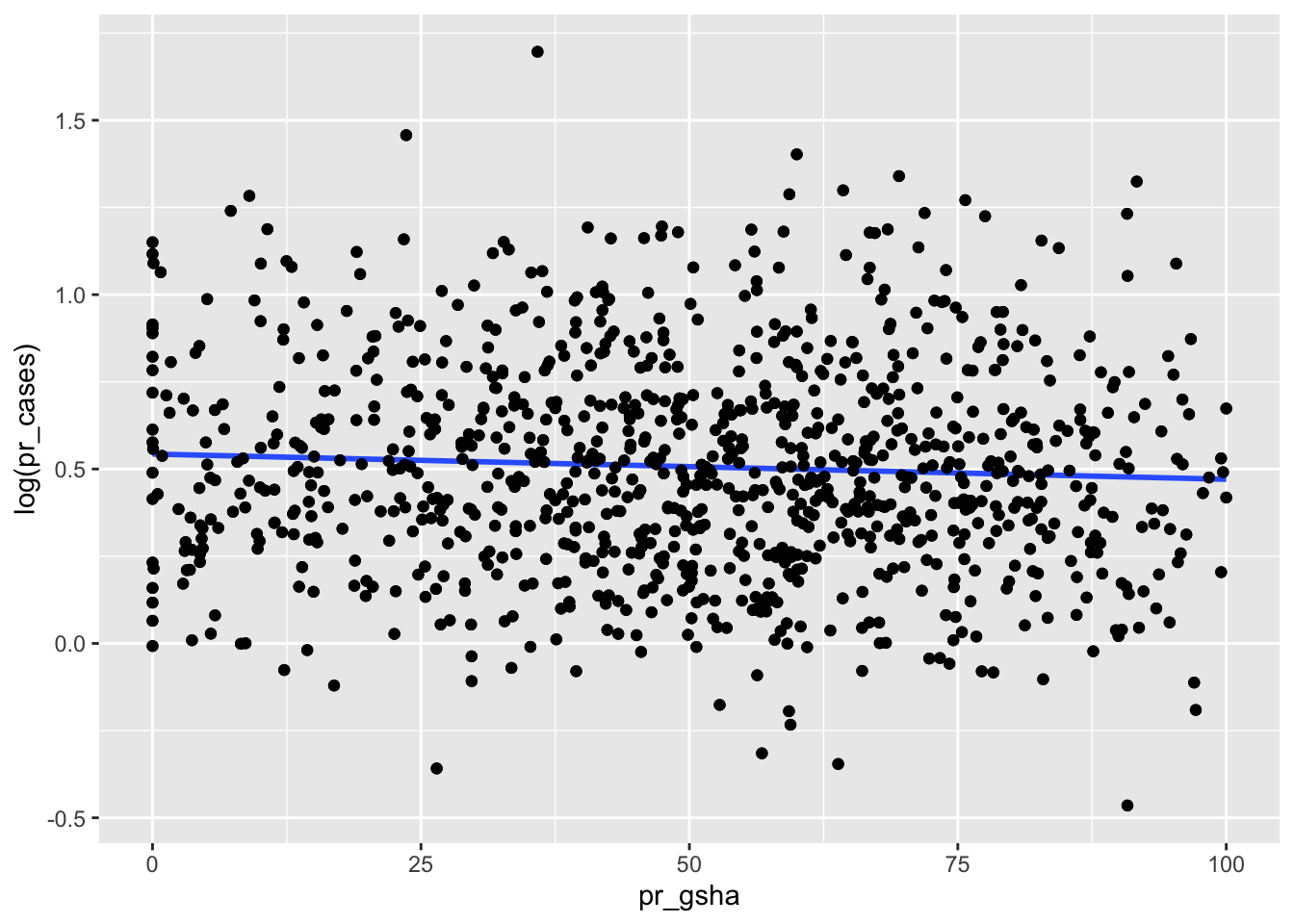

And the OLS model results do not show anything significant at the 95% confidence level:

Regression_data1 <- data%>%
  dplyr::select(c(pr_cases, pr_gsha))

model1 <- Regression_data1%>%
  lm(log(pr_cases) ~
       pr_gsha,
     data=.)

summary(model1)

## 
## Call:
## lm(formula = log(pr_cases) ~ pr_gsha, data = .)
## 
## Residuals:
##      Min       1Q   Median       3Q      Max 
## -0.94199 -0.21360 -0.01899  0.18543  1.17936 
## 
## Coefficients:
##               Estimate Std. Error t value Pr(>|t|)    
## (Intercept)  0.5430038  0.0219899  24.693   <2e-16 ***
## pr_gsha     -0.0007236  0.0003924  -1.844   0.0655 .  
## ---
## Signif. codes:  0 '***' 0.001 '**' 0.01 '*' 0.05 '.' 0.1 ' ' 1
## 
## Residual standard error: 0.3063 on 981 degrees of freedom
## Multiple R-squared:  0.003454,   Adjusted R-squared:  0.002438 
## F-statistic:   3.4 on 1 and 981 DF,  p-value: 0.0655

Although the bi-variate OLS model does not show a significant relationship between the prevalence of COVID-19 and proportion of proximate public green space for the MSOAs, this doesn’t nullify the contribution of the green space variable in a multi-variate OLS model. In fact when a multi-variate model is run and includes the green space variable, the variable is highlighted as significant. We will explore this here as well as creating a multi-variate model without the green space variable so we can observe its contribution to the model.

Stage 1 - Run first model with selected explanatory variables

#Variables selected for multi-variate OLS model 1
mlr_data <- data%>%
  dplyr::select(pop_den, av_hhsz, pct_65, p_hhwdc, p_1phh, pct_bam,
                pct_oo, pct_srn, pct_det, pct_flt, pct_sem, pct_trr,
                pct_ql4, pct_eco_i, pct_limlt, pct_lmltt,pct_ntl,
                pct_h_vb, pct_h_b, pct_h_f, pct_obe, le_m, pr_gsha, pr_cases)

#Multi-variate regression WITH pr_gsha
mlr_1 <- lm(log(pr_cases) ~
              pop_den + av_hhsz + pct_65 + p_hhwdc + p_1phh + pct_bam +
              pct_oo + pct_srn + pct_det + pct_flt + pct_sem + pct_trr +
              pct_ql4 + pct_eco_i + pct_limlt + pct_lmltt + pct_ntl +
              pct_h_vb + pct_h_b + pct_h_f + pct_obe + le_m + pr_gsha,
            data=mlr_data)

summary(mlr_1)

## 
## Call:
## lm(formula = log(pr_cases) ~ pop_den + av_hhsz + pct_65 + p_hhwdc + 
##     p_1phh + pct_bam + pct_oo + pct_srn + pct_det + pct_flt + 
##     pct_sem + pct_trr + pct_ql4 + pct_eco_i + pct_limlt + pct_lmltt + 
##     pct_ntl + pct_h_vb + pct_h_b + pct_h_f + pct_obe + le_m + 
##     pr_gsha, data = mlr_data)
## 
## Residuals:
##      Min       1Q   Median       3Q      Max 
## -0.86400 -0.16919  0.00257  0.16549  1.15375 
## 
## Coefficients:
##               Estimate Std. Error t value Pr(>|t|)    
## (Intercept)  6.8772032 16.0693340   0.428 0.668769    
## pop_den     -0.0007904  0.0002744  -2.880 0.004063 ** 
## av_hhsz      0.4217169  0.1028281   4.101 4.46e-05 ***
## pct_65      -0.0253452  0.0099608  -2.544 0.011099 *  
## p_hhwdc     -0.0085399  0.0036539  -2.337 0.019634 *  
## p_1phh      -0.0004455  0.0040601  -0.110 0.912647    
## pct_bam     -0.0039761  0.0011061  -3.595 0.000341 ***
## pct_oo       0.0080370  0.0045609   1.762 0.078366 .  
## pct_srn     -0.0089997  0.0015241  -5.905 4.89e-09 ***
## pct_det     -0.0385391  0.0243386  -1.583 0.113648    
## pct_flt     -0.0313295  0.0241886  -1.295 0.195556    
## pct_sem     -0.0357779  0.0241593  -1.481 0.138957    
## pct_trr     -0.0374254  0.0241929  -1.547 0.122203    
## pct_ql4     -0.0099605  0.0028522  -3.492 0.000501 ***
## pct_eco_i    0.0116071  0.0033758   3.438 0.000611 ***
## pct_limlt    0.0043868  0.1580796   0.028 0.977867    
## pct_lmltt   -0.0389557  0.1581199  -0.246 0.805450    
## pct_ntl     -0.0268940  0.1580897  -0.170 0.864953    
## pct_h_vb    -0.0324920  0.0492071  -0.660 0.509213    
## pct_h_b      0.0724962  0.0310336   2.336 0.019693 *  
## pct_h_f     -0.0201445  0.0184603  -1.091 0.275443    
## pct_obe      0.0010391  0.0044963   0.231 0.817290    
## le_m        -0.0094672  0.0036513  -2.593 0.009664 ** 
## pr_gsha     -0.0008406  0.0003494  -2.406 0.016312 *  
## ---
## Signif. codes:  0 '***' 0.001 '**' 0.01 '*' 0.05 '.' 0.1 ' ' 1
## 
## Residual standard error: 0.2542 on 959 degrees of freedom
## Multiple R-squared:  0.3289, Adjusted R-squared:  0.3128 
## F-statistic: 20.43 on 23 and 959 DF,  p-value: < 2.2e-16

The results in this model show that in a multi-variate model the pr_gsha variable is significant with a p-value of 0.016312. Several variables have been flagged as significant in the model so model 2 will drop any insignificant variables.

Stage 2 - Run second multi-variate OLS model

#Only selected the significant variables from model_1
mlr_data_2 <- data%>%
  dplyr::select(pop_den, av_hhsz, pct_65, p_hhwdc, pct_bam,
                pct_srn, pct_ql4, pct_eco_i, pct_h_b,le_m, pr_gsha, pr_cases)

#model 2 - with pr_gsha variable
mlr_2 <- lm(log(pr_cases) ~ pop_den + av_hhsz + pct_65 + p_hhwdc + pct_bam +
              pct_srn + pct_ql4 + pct_eco_i + pct_h_b + le_m + pr_gsha, 
            data=mlr_data_2)
            
summary(mlr_2)

## 
## Call:
## lm(formula = log(pr_cases) ~ pop_den + av_hhsz + pct_65 + p_hhwdc + 
##     pct_bam + pct_srn + pct_ql4 + pct_eco_i + pct_h_b + le_m + 
##     pr_gsha, data = mlr_data_2)
## 
## Residuals:
##      Min       1Q   Median       3Q      Max 
## -0.91674 -0.16987 -0.00386  0.16328  1.19513 
## 
## Coefficients:
##               Estimate Std. Error t value Pr(>|t|)    
## (Intercept)  0.5989026  0.3073364   1.949 0.051620 .  
## pop_den     -0.0004593  0.0002593  -1.772 0.076785 .  
## av_hhsz      0.3129210  0.0633937   4.936 9.37e-07 ***
## pct_65      -0.0197141  0.0038043  -5.182 2.67e-07 ***
## p_hhwdc     -0.0112946  0.0035257  -3.203 0.001402 ** 
## pct_bam     -0.0033661  0.0009034  -3.726 0.000206 ***
## pct_srn     -0.0081800  0.0010299  -7.943 5.45e-15 ***
## pct_ql4     -0.0047892  0.0013228  -3.621 0.000309 ***
## pct_eco_i    0.0162708  0.0027251   5.971 3.31e-09 ***
## pct_h_b      0.0622418  0.0173350   3.591 0.000347 ***
## le_m        -0.0074060  0.0034849  -2.125 0.033823 *  
## pr_gsha     -0.0010201  0.0003437  -2.968 0.003073 ** 
## ---
## Signif. codes:  0 '***' 0.001 '**' 0.01 '*' 0.05 '.' 0.1 ' ' 1
## 
## Residual standard error: 0.2592 on 971 degrees of freedom
## Multiple R-squared:  0.2936, Adjusted R-squared:  0.2856 
## F-statistic: 36.68 on 11 and 971 DF,  p-value: < 2.2e-16

The new model shows that all the variables except the pop_den variable are significant in the model. The model shows that pr_gsha is a negative coefficient, meaning that at a global scale when the proportion of greenspace increases, a decrease in the prevalence of COVID-19 is experienced. The R^2 is still on the low end at 0.29 and 0.28 (for adj r-sq) but we can conclude that the variables in the model do explain some of the variation in the proportion of COVID-19 variable.

To meet the conditions of a global regression model, the model needed to be checked for multicollinearity between the variables.

The av_hhsz had the highest VIF at 6.5 however since it is under the threshold of 10 we will keep it in the model.

Stage 3 - Finalising the multi-variate OLS model

#Finalise model and drop pop_den variable

final_data <- data%>%
  dplyr::select(code, av_hhsz, pct_65, p_hhwdc, pct_bam,
                pct_srn, pct_ql4, pct_eco_i, pct_h_b,le_m, pr_gsha, pr_cases)

mlr_final <- lm(log(pr_cases) ~ av_hhsz + pct_65 + p_hhwdc + pct_bam +
                  pct_srn + pct_ql4 + pct_eco_i + pct_h_b + le_m + pr_gsha, 
                data=final_data)

summary(mlr_final)

## 
## Call:
## lm(formula = log(pr_cases) ~ av_hhsz + pct_65 + p_hhwdc + pct_bam + 
##     pct_srn + pct_ql4 + pct_eco_i + pct_h_b + le_m + pr_gsha, 
##     data = final_data)
## 
## Residuals:
##      Min       1Q   Median       3Q      Max 
## -0.92217 -0.16943 -0.00424  0.16351  1.23901 
## 
## Coefficients:
##               Estimate Std. Error t value Pr(>|t|)    
## (Intercept)  0.6546595  0.3060567   2.139 0.032683 *  
## av_hhsz      0.2947033  0.0626228   4.706 2.89e-06 ***
## pct_65      -0.0174522  0.0035876  -4.865 1.34e-06 ***
## p_hhwdc     -0.0101099  0.0034655  -2.917 0.003612 ** 
## pct_bam     -0.0032547  0.0009022  -3.607 0.000325 ***
## pct_srn     -0.0082656  0.0010299  -8.026 2.90e-15 ***
## pct_ql4     -0.0055798  0.0012466  -4.476 8.51e-06 ***
## pct_eco_i    0.0159194  0.0027208   5.851 6.67e-09 ***
## pct_h_b      0.0557567  0.0169627   3.287 0.001049 ** 
## le_m        -0.0079763  0.0034738  -2.296 0.021878 *  
## pr_gsha     -0.0009165  0.0003391  -2.703 0.006994 ** 
## ---
## Signif. codes:  0 '***' 0.001 '**' 0.01 '*' 0.05 '.' 0.1 ' ' 1
## 
## Residual standard error: 0.2595 on 972 degrees of freedom
## Multiple R-squared:  0.2913, Adjusted R-squared:  0.284 
## F-statistic: 39.95 on 10 and 972 DF,  p-value: < 2.2e-16

Running VIF again to check for multicollinearity:

VIF(mlr_final)

##   av_hhsz    pct_65   p_hhwdc   pct_bam   pct_srn   pct_ql4 pct_eco_i   pct_h_b      le_m   pr_gsha 
##  6.341802  3.189459  4.585663  4.427108  4.239891  3.170195  2.682487  4.248122  1.928769  1.040019

The VIF results are acceptable and the 10 explanatory variables all remain significant in the model.

Stage 4 - Creating the final model without the proportion of proximate green space variable

#Final model WITHOUT the pr_gsha variable
mlr_final2 <- lm(log(pr_cases) ~ av_hhsz + pct_65 + p_hhwdc + pct_bam +
                   pct_srn + pct_ql4 + pct_eco_i + pct_h_b + le_m, 
                 data=final_data)

summary(mlr_final2)

## 
## Call:
## lm(formula = log(pr_cases) ~ av_hhsz + pct_65 + p_hhwdc + pct_bam + 
##     pct_srn + pct_ql4 + pct_eco_i + pct_h_b + le_m, data = final_data)
## 
## Residuals:
##      Min       1Q   Median       3Q      Max 
## -0.95336 -0.16851 -0.00658  0.16536  1.24825 
## 
## Coefficients:
##              Estimate Std. Error t value Pr(>|t|)    
## (Intercept)  0.684555   0.306846   2.231 0.025912 *  
## av_hhsz      0.285313   0.062729   4.548 6.09e-06 ***
## pct_65      -0.017392   0.003599  -4.832 1.57e-06 ***
## p_hhwdc     -0.010796   0.003467  -3.113 0.001903 ** 
## pct_bam     -0.003216   0.000905  -3.554 0.000398 ***
## pct_srn     -0.008518   0.001029  -8.278 4.10e-16 ***
## pct_ql4     -0.005641   0.001250  -4.511 7.24e-06 ***
## pct_eco_i    0.016406   0.002724   6.023 2.42e-09 ***
## pct_h_b      0.055725   0.017018   3.275 0.001096 ** 
## le_m        -0.008585   0.003478  -2.469 0.013731 *  
## ---
## Signif. codes:  0 '***' 0.001 '**' 0.01 '*' 0.05 '.' 0.1 ' ' 1
## 
## Residual standard error: 0.2603 on 973 degrees of freedom
## Multiple R-squared:  0.2859, Adjusted R-squared:  0.2793 
## F-statistic: 43.29 on 9 and 973 DF,  p-value: < 2.2e-16

When comparing the results we can see that the pr_gsha has a tiny coefficient however it does add to the r-squared value. Then again, the r-squared value will always increase when adding a new variable to the model. When we compare the adjusted R^2 we can see that it has ever so slightly improved the model by including the pr_gsha variable. We can say that the proportion of proximate public green space does add to the model and we should explore the model further using spatial statistical analyses.

Let’s save the residual results from the global mlr_final model and write them out

mlr_final_data <- mlr_final %>%
  broom::augment(., final_data)

# add the residuals backs to the data sf 
data <- data %>%
  mutate(final_model_resids = residuals(mlr_final))

Exploring the spatial autocorrelation of the multi-variate residuals

From the Moran’s I, Geary’s C and Getis-Ords statistics we observed earlier, we quantified the spatial autocorrelation that exists in the the pr_gsha variable. This spatial autocorrelation biases the model and will need to be dealt with.

We’ll plot the residuals of the model to see what the obvious patterns are:

tmap_mode("view")

## tmap mode set to interactive viewing

final_resids_pal <- rev(brewer.pal(5, "RdYlBu"))

tm_shape(data) +
  tm_polygons("final_model_resids",
              palette = final_resids_pal)

## Variable(s) "final_model_resids" contains positive and negative values, so midpoint is set to 0. Set midpoint = NA to show the full spectrum of the color palette.

This plot visually confirms spatial autocorrelation of the final_mlr residuals but we can run Moran’s I to quantify that spatial autocorrelation exists between the residuals.

We can use the same centroids, neighbours and spatial weights matrix parameters we made earlier for this:

• coordsMSOA

• msoa.lw

• msoa_nb

#Creating
Queen_MI <- data %>%
  st_drop_geometry()%>%
  dplyr::select(final_model_resids)%>%
  pull()%>%
  moran.test(., msoa.lw)%>%
  tidy()
Queen_MI

## # A tibble: 1 x 7
##   estimate1 estimate2 estimate3 statistic   p.value method                           alternative
##       <dbl>     <dbl>     <dbl>     <dbl>     <dbl> <chr>                            <chr>      
## 1     0.460  -0.00102  0.000352      24.6 1.25e-133 Moran I test under randomisation greater

The results show that Queen_MI is about 0.460 this shows that there’s moderate spatial autocorrelation between our residuals and therefore it is likely to be biasing our final multi-variate model.

This suggests that the multi-variate model is inappropriate for accurately exploring our spatial data and the associations which exist between COVID-19 prevalence and the various explanatory variables (including the proportion of proximate public green space)

This finding means we can move onto creating a Spatial Lag Model (SLM) and Spatial Error Model (SEM) to explore the impact of spatial autocorrelation in the multi-variate model.

Spatial Lag Model

The Lag Model test results are significant wiht a p-value of < 0.05. This means we can reject the null hypothesis that there is no spatial autocorrelation between our final model residuals

#what do the outputs show? #The RHO #The LR

We can run Moran’s I on the SLM residuals to observe the removal of spatial autocorrelation:

#Running the Moran's I on the SLM residuals
QMoran <- data %>%
  st_drop_geometry()%>%
  dplyr::select(slm_q_resids)%>%
  pull()%>%
  moran.test(., msoa.lw)%>%
  tidy()

QMoran

## # A tibble: 1 x 7
##   estimate1 estimate2 estimate3 statistic  p.value method                           alternative
##       <dbl>     <dbl>     <dbl>     <dbl>    <dbl> <chr>                            <chr>      
## 1    0.0577  -0.00102  0.000352      3.13 0.000864 Moran I test under randomisation greater

Using the Queens spatial weights matrix and running Moran’s I we can see the removal of spatial autocorrelation since the Moran’s I statistic is 0.0577.

Spatial Error Model EXPLAIN RESULTS

#Use queen contiguity neighbours too
sem_final_model_q <- errorsarlm(log(pr_cases) ~ av_hhsz + pct_65 + p_hhwdc + pct_bam +
                                  pct_srn + pct_ql4 + pct_eco_i + pct_h_b + le_m + pr_gsha,
                                data = final_data,
                                nb2listw(msoa_nb, style="C"), 
                                method = "eigen")

tidy(sem_final_model_q)

## # A tibble: 12 x 5
##    term         estimate std.error statistic  p.value
##    <chr>           <dbl>     <dbl>     <dbl>    <dbl>
##  1 (Intercept)  1.24      0.275        4.51  6.43e- 6
##  2 av_hhsz      0.0913    0.0637       1.43  1.52e- 1
##  3 pct_65      -0.00659   0.00356     -1.85  6.42e- 2
##  4 p_hhwdc     -0.00842   0.00346     -2.43  1.50e- 2
##  5 pct_bam     -0.000359  0.00107     -0.336 7.37e- 1
##  6 pct_srn     -0.00658   0.00104     -6.31  2.86e-10
##  7 pct_ql4     -0.00806   0.00157     -5.13  2.92e- 7
##  8 pct_eco_i    0.00734   0.00302      2.43  1.50e- 2
##  9 pct_h_b      0.0126    0.0158       0.796 4.26e- 1
## 10 le_m        -0.00728   0.00289     -2.52  1.18e- 2
## 11 pr_gsha     -0.000583  0.000281    -2.08  3.80e- 2
## 12 lambda       0.689     0.0273      25.2   0.

sem_final_model_q

## 
## Call:
## errorsarlm(formula = log(pr_cases) ~ av_hhsz + pct_65 + p_hhwdc + 
##     pct_bam + pct_srn + pct_ql4 + pct_eco_i + pct_h_b + le_m + 
##     pr_gsha, data = final_data, listw = nb2listw(msoa_nb, style = "C"), 
##     method = "eigen")
## Type: error 
## 
## Coefficients:
##        lambda   (Intercept)       av_hhsz        pct_65       p_hhwdc       pct_bam       pct_srn       pct_ql4 
##  0.6891495628  1.2387859267  0.0912501727 -0.0065865121 -0.0084180427 -0.0003587762 -0.0065769863 -0.0080575504 
##     pct_eco_i       pct_h_b          le_m       pr_gsha 
##  0.0073411936  0.0125657831 -0.0072751890 -0.0005832152 
## 
## Log likelihood: 141.6084

From looking at the SLM and SEM results it could be that the spatial autocorrelation is biasing the final multi-variate OLS model but it also could be that the global regression models are ultimately unsuitable for the data we are exploring.

A Geographically Weighted Regression may be more suitable to investigate the local story, for example in some areas the slope coefficients between the dependent and independent variables may differ. Global models fail to detect this spatial variation. We can explore this by carrying out a GWR.

Let’s print the results of the final multi-variate OLS model and quickly plot them:

summary(mlr_final)

## 
## Call:
## lm(formula = log(pr_cases) ~ av_hhsz + pct_65 + p_hhwdc + pct_bam + 
##     pct_srn + pct_ql4 + pct_eco_i + pct_h_b + le_m + pr_gsha, 
##     data = final_data)
## 
## Residuals:
##      Min       1Q   Median       3Q      Max 
## -0.92217 -0.16943 -0.00424  0.16351  1.23901 
## 
## Coefficients:
##               Estimate Std. Error t value Pr(>|t|)    
## (Intercept)  0.6546595  0.3060567   2.139 0.032683 *  
## av_hhsz      0.2947033  0.0626228   4.706 2.89e-06 ***
## pct_65      -0.0174522  0.0035876  -4.865 1.34e-06 ***
## p_hhwdc     -0.0101099  0.0034655  -2.917 0.003612 ** 
## pct_bam     -0.0032547  0.0009022  -3.607 0.000325 ***
## pct_srn     -0.0082656  0.0010299  -8.026 2.90e-15 ***
## pct_ql4     -0.0055798  0.0012466  -4.476 8.51e-06 ***
## pct_eco_i    0.0159194  0.0027208   5.851 6.67e-09 ***
## pct_h_b      0.0557567  0.0169627   3.287 0.001049 ** 
## le_m        -0.0079763  0.0034738  -2.296 0.021878 *  
## pr_gsha     -0.0009165  0.0003391  -2.703 0.006994 ** 
## ---
## Signif. codes:  0 '***' 0.001 '**' 0.01 '*' 0.05 '.' 0.1 ' ' 1
## 
## Residual standard error: 0.2595 on 972 degrees of freedom
## Multiple R-squared:  0.2913, Adjusted R-squared:  0.284 
## F-statistic: 39.95 on 10 and 972 DF,  p-value: < 2.2e-16

tm_shape(data) +
  tm_polygons("final_model_resids",
              palette = final_resids_pal)

## Variable(s) "final_model_resids" contains positive and negative values, so midpoint is set to 0. Set midpoint = NA to show the full spectrum of the color palette.

For the spgwr package I will be using, we will need to transform our final_data for the regression and the MSOA centroids into sp objects from sf:

Next we need to calculate the kernel bandwidth for the GWR. This may take several moments to configure - … EXPLAIN

GWRbandwidth <- gwr.sel(log(pr_cases) ~ av_hhsz + pct_65 + p_hhwdc + pct_bam +
                          pct_srn + pct_ql4 + pct_eco_i + pct_h_b + le_m + pr_gsha, 
                        data=final_data_SP, 
                        coords=coordsMSOA_SP,
                        adapt=T)

## Warning in gwr.sel(log(pr_cases) ~ av_hhsz + pct_65 + p_hhwdc + pct_bam + : data is Spatial* object, ignoring coords
## argument

## Adaptive q: 0.381966 CV score: 59.67584 
## Adaptive q: 0.618034 CV score: 62.75719 
## Adaptive q: 0.236068 CV score: 55.80362 
## Adaptive q: 0.145898 CV score: 51.26128 
## Adaptive q: 0.09016994 CV score: 46.85088 
## Adaptive q: 0.05572809 CV score: 43.51028 
## Adaptive q: 0.03444185 CV score: 41.41683 
## Adaptive q: 0.02128624 CV score: 40.30218 
## Adaptive q: 0.01315562 CV score: 41.00101 
## Adaptive q: 0.02258059 CV score: 40.32868 
## Adaptive q: 0.02102684 CV score: 40.29492 
## Adaptive q: 0.0180203 CV score: 40.27604 
## Adaptive q: 0.01905083 CV score: 40.26635 
## Adaptive q: 0.01912801 CV score: 40.26746 
## Adaptive q: 0.01875441 CV score: 40.26363 
## Adaptive q: 0.018474 CV score: 40.26355 
## Adaptive q: 0.01860461 CV score: 40.26326 
## Adaptive q: 0.0186453 CV score: 40.26329 
## Adaptive q: 0.01856392 CV score: 40.26329 
## Adaptive q: 0.01860461 CV score: 40.26326

The GWR can now be run:

gwr.model = gwr(log(pr_cases) ~ av_hhsz + pct_65 + p_hhwdc + pct_bam +
                  pct_srn + pct_ql4 + pct_eco_i + pct_h_b + le_m + pr_gsha, 
                data=final_data_SP, 
                coords=coordsMSOA_SP, 
                adapt=GWRbandwidth, 
                hatmatrix=TRUE, 
                se.fit=TRUE)

## Warning in gwr(log(pr_cases) ~ av_hhsz + pct_65 + p_hhwdc + pct_bam + pct_srn + : data is Spatial* object, ignoring coords
## argument

## Warning in proj4string(data): CRS object has comment, which is lost in output

## Warning in showSRID(uprojargs, format = "PROJ", multiline = "NO", prefer_proj = prefer_proj): Discarded datum Unknown based
## on Airy 1830 ellipsoid in CRS definition

gwr.model

## Call:
## gwr(formula = log(pr_cases) ~ av_hhsz + pct_65 + p_hhwdc + pct_bam + 
##     pct_srn + pct_ql4 + pct_eco_i + pct_h_b + le_m + pr_gsha, 
##     data = final_data_SP, coords = coordsMSOA_SP, adapt = GWRbandwidth, 
##     hatmatrix = TRUE, se.fit = TRUE)
## Kernel function: gwr.Gauss 
## Adaptive quantile: 0.01860461 (about 18 of 983 data points)
## Summary of GWR coefficient estimates at data points:
##                     Min.     1st Qu.      Median     3rd Qu.        Max.  Global
## X.Intercept. -1.7154e+00  4.7777e-01  1.1481e+00  1.8057e+00  6.4479e+00  0.6547
## av_hhsz      -8.0306e-01 -1.4321e-01  8.3513e-02  2.5849e-01  9.9795e-01  0.2947
## pct_65       -1.1271e-01 -2.2558e-02 -1.3163e-02  2.2242e-04  3.7835e-02 -0.0175
## p_hhwdc      -6.0291e-02 -1.8679e-02 -5.4315e-03  6.7150e-03  3.8865e-02 -0.0101
## pct_bam      -2.0100e-02 -5.7978e-03  5.1545e-05  4.1802e-03  1.2897e-02 -0.0033
## pct_srn      -2.0614e-02 -9.1760e-03 -4.6759e-03 -8.9053e-04  7.5921e-03 -0.0083
## pct_ql4      -3.0206e-02 -1.1307e-02 -7.2343e-03 -1.6972e-03  2.2237e-02 -0.0056
## pct_eco_i    -3.5533e-02 -1.0235e-04  8.7503e-03  1.7120e-02  7.2301e-02  0.0159
## pct_h_b      -1.9605e-01 -5.0199e-02 -5.8074e-03  6.2524e-02  2.5810e-01  0.0558
## le_m         -3.6816e-02 -1.3982e-02 -6.0231e-03  2.3828e-04  2.4850e-02 -0.0080
## pr_gsha      -4.1502e-03 -7.7598e-04 -1.3693e-04  4.2710e-04  2.1984e-03 -0.0009
## Number of data points: 983 
## Effective number of parameters (residual: 2traceS - traceS'S): 290.1353 
## Effective degrees of freedom (residual: 2traceS - traceS'S): 692.8647 
## Sigma (residual: 2traceS - traceS'S): 0.1891109 
## Effective number of parameters (model: traceS): 209.6028 
## Effective degrees of freedom (model: traceS): 773.3972 
## Sigma (model: traceS): 0.1789944 
## Sigma (ML): 0.1587684 
## AICc (GWR p. 61, eq 2.33; p. 96, eq. 4.21): -291.6669 
## AIC (GWR p. 96, eq. 4.22): -618.8112 
## Residual sum of squares: 24.77887 
## Quasi-global R2: 0.7316511

Lets write the regression coefficients back to the final_data object. We can plot these coefficients shortly:

results <- as.data.frame(gwr.model$SDF)

final_data <- final_data%>%
  mutate(coef_av_hhsz = results$av_hhsz,
         coef_pct_65 = results$pct_65,
         coef_p_hhwdc = results$p_hhwdc,
         coef_pct_bam = results$pct_bam,
         coef_pct_srn = results$pct_srn,
         coef_pct_ql4 = results$pct_ql4,
         coef_pct_eco_i = results$pct_eco_i,
         coef_pct_h_b = results$pct_h_b,
         coef_le_m = results$le_m,
         coef_pr_gsha = results$pr_gsha)

We can then merge the GWR coefficient results with the original sf dataframe:

##Add the GWR coefficients back to the original data sf object
#Drop geometry from final_data first
final_data <- final_data%>%
  st_drop_geometry()%>%
  dplyr::select(c(code,
                  coef_av_hhsz,
                  coef_pct_65,
                  coef_p_hhwdc,
                  coef_pct_bam,
                  coef_pct_srn,
                  coef_pct_ql4,
                  coef_pct_eco_i,
                  coef_pct_h_b,
                  coef_le_m,
                  coef_pr_gsha))

data <- data%>%
  merge(., final_data,
        by.x=1,
        by.y=1)

First plot of the GWR coefficients for proportion of proximate green space variable

#Plotting the pr_gsha GWR residuals
tmap_mode("plot")

## tmap mode set to plotting

tm_shape(data) +
  tm_polygons(col = "coef_pr_gsha", 
              palette = "RdBu", 
              alpha = 0.5)

## Variable(s) "coef_pr_gsha" contains positive and negative values, so midpoint is set to 0. Set midpoint = NA to show the full spectrum of the color palette.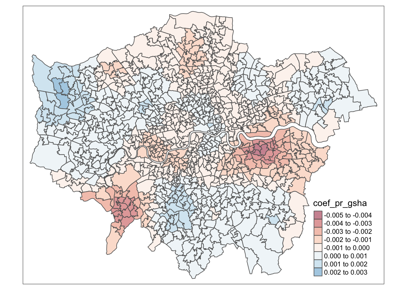

Visualisation and Cartography

This final part of the methodology will be dedicated to making the data visualisations and maps that are included in the write-up.

The following visualisations will be made:

• Basic map of the London MSOA boundaries

• Histogram of the proportion of COVID-19 in London MSOAs

• Histogram of the proportion of proximate green space in London MSOAs

• Map of the proportion of proximate green space in London MSOAs

• Map of the GWR coefficients for the proportion of proximate green space across London

ggsave() should work for saving any ggplot but for me it didn’t work so I have been using a function found here. All credit to enricoferrero on stackoverflow!

Load libraries we need:

Basic map of London MSOA boundaries:

tmap_mode("plot")

## tmap mode set to plotting

boundaries <- tm_shape(data) +
  tm_polygons(col ="blue",
              alpha = 0.1,
              border.lwd = 0.3)+
  tm_layout(inner.margins = c(0.09, 0.10, 0.10, 0.10))+
  tm_compass(text.size = 0.5,
             position = c("right", "top"))+
  tm_scale_bar(text.size = 0.4,
               color.dark = "gray60",
                   position = c("left", "BOTTOM")) +
  tm_layout(title = "London's 983 Middle Super Output Areas (MSOA)", title.size = 0.8) +
  tm_credits(size = 3, text = "Contains National Statistics data © Crown copyright and database right [2015] and Contains Ordnance Survey data © Crown copyright and database right [2015]\nMap created by Isabella Brant", position = c("left", "BOTTOM"))

boundaries 

#tmap_save(boundaries, filename="msoa_map.png")

Histogram of the proportion of proximate green space in London MSOAs:

greenspace_dist <- data%>%
  ggplot(aes(x=pr_gsha)) +
  geom_histogram(position="identity", 
                 alpha=0.5, 
                 bins=15, 
                 fill="lightblue2", col="lightblue2")+
  geom_vline(aes(xintercept=mean(pr_gsha)),
             color="blue",
             linetype="dashed")+
  labs(title="Distribution of the proportion\nof proximate public green spaces to the total\n land area of London MSOAs.",
       x="Proportion of proximate public green space",
       y="Frequency")+
  theme_classic()+
  theme(plot.title = element_text(hjust = 0.5))

greenspace_dist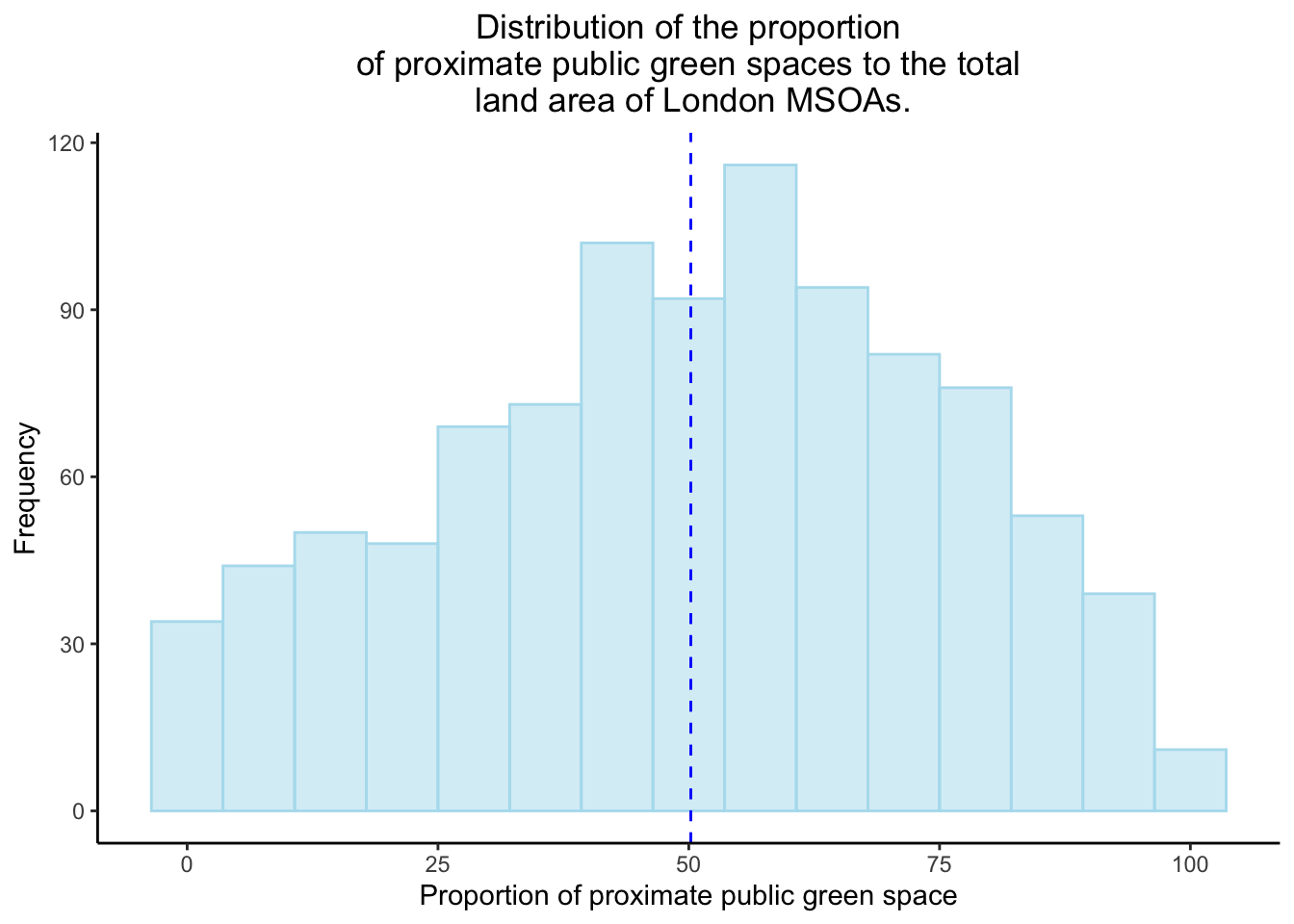

#savePlot <- function(greenspace_dist) {
        #pdf("greenspace_dist.pdf")
        #print(greenspace_dist)
        #dev.off()
#}

#savePlot(greenspace_dist)

Histogram of the proportion of COVID-19 in London MSOAs:

covid_dist <- data%>%
  ggplot(aes(x=pr_cases)) +
  geom_histogram(position="identity", 
                 alpha=0.5, 
                 bins=15, 
                 fill="lightblue2", col="lightblue3")+
  geom_vline(aes(xintercept=mean(pr_cases)),
             color="blue",
             linetype="dashed")+
  labs(title="Distribution of the proportion of total COVID-19 cases to the population
       of each MSOA.",
       x="Proportion of COVID-19 cases (%)",
       y="Frequency")+
  theme_classic()+
  theme(plot.title = element_text(hjust = 0.5))

covid_dist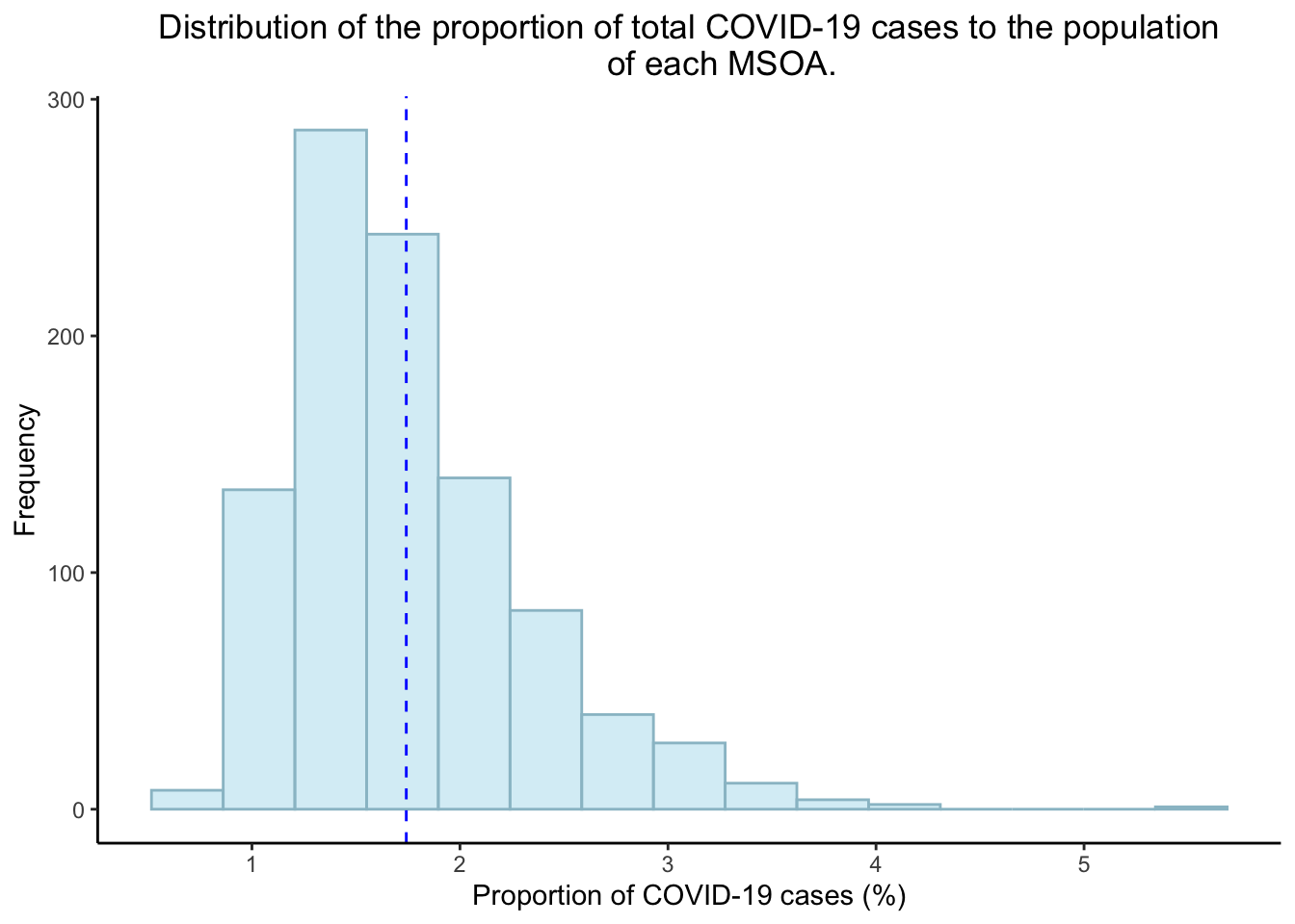

#savePlot <- function(covid_dist) {
        #pdf("covid_dist.pdf")
        #print(covid_dist)
        #dev.off()
#}

#savePlot(covid_dist)

Map of the proportion of proximate green space in London MSOAs:

gs_pal <- brewer.pal(5, "Greens")
  
prop_gs <- tm_shape(data) +
  tm_polygons("pr_gsha",
              text.size = 0.4,
              palette = gs_pal,
              title="Proportion of green space (%)",
              title.size = 0.3,
              alpha = 0.8)+
  tm_layout(inner.margins = c(0.10, 0.18, 0.12, 0.20))+
  tm_compass(text.size = 0.5,
             position = c("right", "top"))+
  tm_scale_bar(text.size = 0.4,
               color.dark = "gray60",
                   position = c("left", "BOTTOM")) +
  tm_layout(title = "Proportion of proximate public green space to the total\nland area of each London MSOA.", title.size = 1) +
  tm_credits(size = 3, text = "Contains National Statistics data © Crown copyright and database right [2015] and Contains Ordnance Survey data © Crown copyright and database right [2015]\nMap created by Isabella Brant", position = c("left", "BOTTOM"))

prop_gs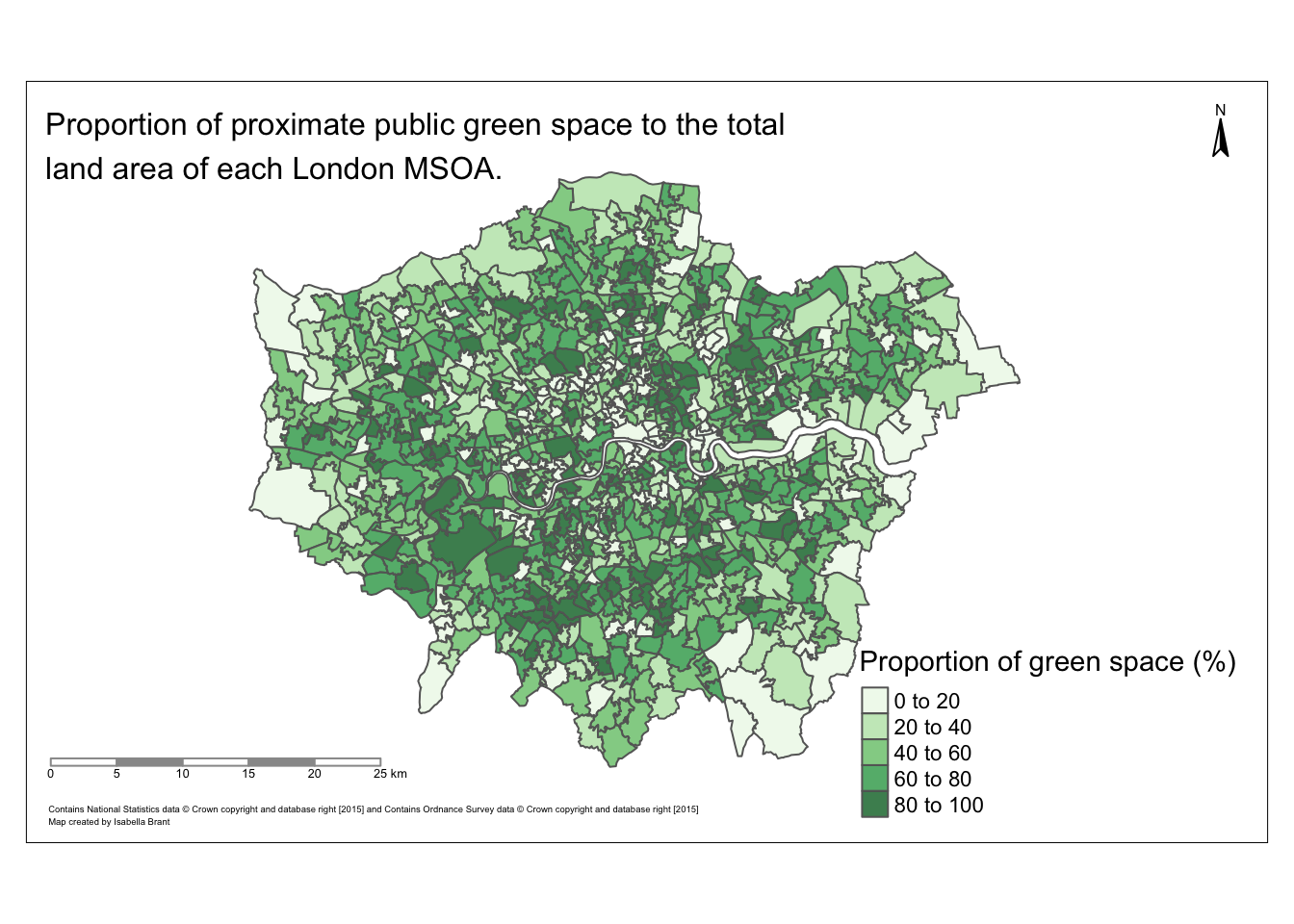

#tmap_save(prop_gs, filename="prop_gs.png")

Map of the GWR coefficients for the proportion of proximate green space across London:

tmap_mode("plot")

## tmap mode set to plotting

GWR_map <- tm_shape(data) +
  tm_polygons("coef_pr_gsha",
              text.size = 0.4,
              palette = "RdBu",
              title="Coefficient value",
              title.size = 0.3,
              alpha = 0.6)+
  tm_layout(inner.margins = c(0.10, 0.18, 0.12, 0.20))+
  tm_compass(text.size = 0.5,
             position = c("right", "top"))+
  tm_scale_bar(text.size = 0.4,
               color.dark = "gray60",
                   position = c("left", "BOTTOM")) +
  tm_layout(title = "GWR coefficients for the proportion of proximate\ngreen space variable", 
            title.size = 1,
            title.color = "black") +
  tm_credits(size = 3, text = "Contains National Statistics data © Crown copyright and database right [2015] and Contains Ordnance Survey data © Crown copyright and database right [2015]\nMap created by Isabella Brant", position = c("left", "BOTTOM"))

GWR_map

## Variable(s) "coef_pr_gsha" contains positive and negative values, so midpoint is set to 0. Set midpoint = NA to show the full spectrum of the color palette.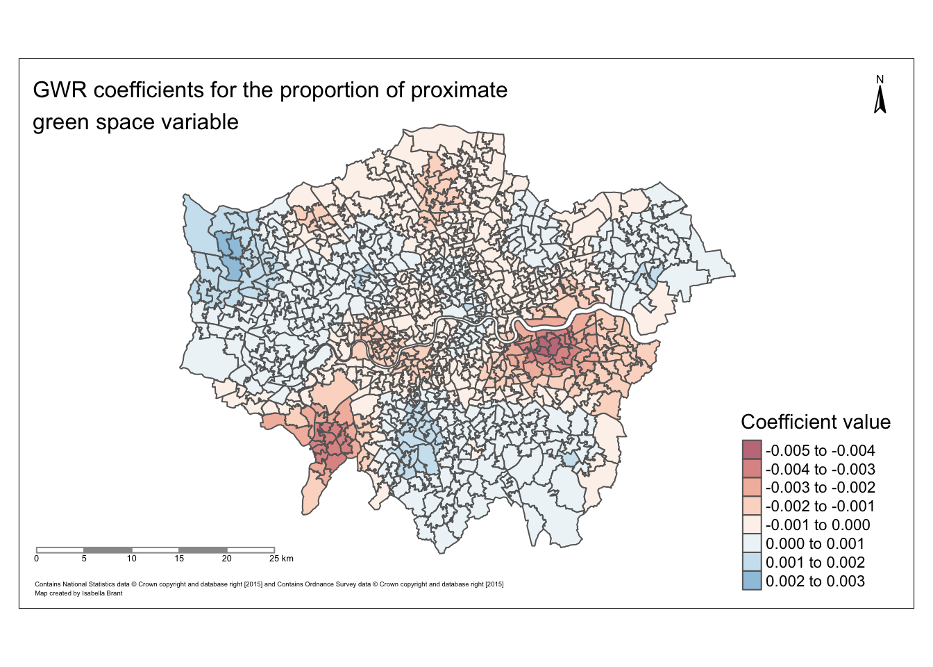

#tmap_save(GWR_map, filename="gwr_map.png")