Chapter 11 Appendix

11.1 About R

History of R

• R is an implementation of the S programming language combined with lexical scoping semantics inspired by Scheme.
• S was created by John Chambers while at Bell Labs.
• There are some important differences, but much of the code written for S runs unaltered.
• R was created by Ross Ihaka and Robert Gentleman at the University of Auckland, New Zealand, and is currently developed by the R Development Core Team, of which Chambers is a member.
• R is named partly after the first names of the first two R authors and partly as a play on the name of S.
• The project was conceived in 1992, with an initial version released in 1995 and a stable beta version in 2000.

Meet R

The Facts

• R is a language and environment for statistical computing and graphics
• Freely available and maintained by volunteers
• R is extensible; can be expanded by installing packages

How to get it

• http://www.r-project.org/
• Available for Windows, Mac, Linux
• Free to install, no catches

Also highly recommended

• R Studio: a free IDE for R
• http://www.rstudio.com/
• If you install R and R Studio, then you only need to run R Studio

Use R

• R is command-line driven (very little point-and-click)
• You use functions to work with data
• Most analyses require writing a script, which is sourced into the R console
• R Studio makes this process easier

What is so special about R?

• Free
• Over 12000 packages that add functionality (about 25 come with R)
• Produces nice print-ready graphics
• Open-source (you can see how it does what it does)
• Easy to install and non-invasive

Text Assumptions, Goals and Expectations

• No experience with R is necessary
• Familiarity with basic statistical concepts
• Get you comfortable enough to start using R
• Give you with example code you can use and resources to learn more
• You will not be an expert after a single course
• You must use R to learn R

11.2 Software Requirements

To install R on a Mac or PC, you first need to go to: http://www.r.project.org

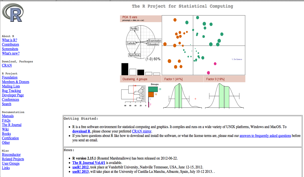
Source: The R project for Statistical Computing.

Select the appropriate Download for your system.

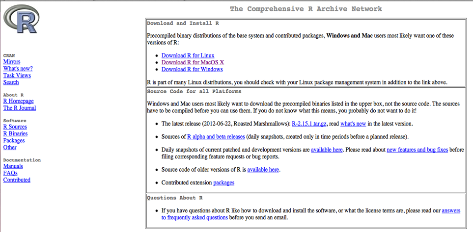
Source: The R project for Statistical Computing.

Select the most recent version of R, not 2.15.1, as shown here.

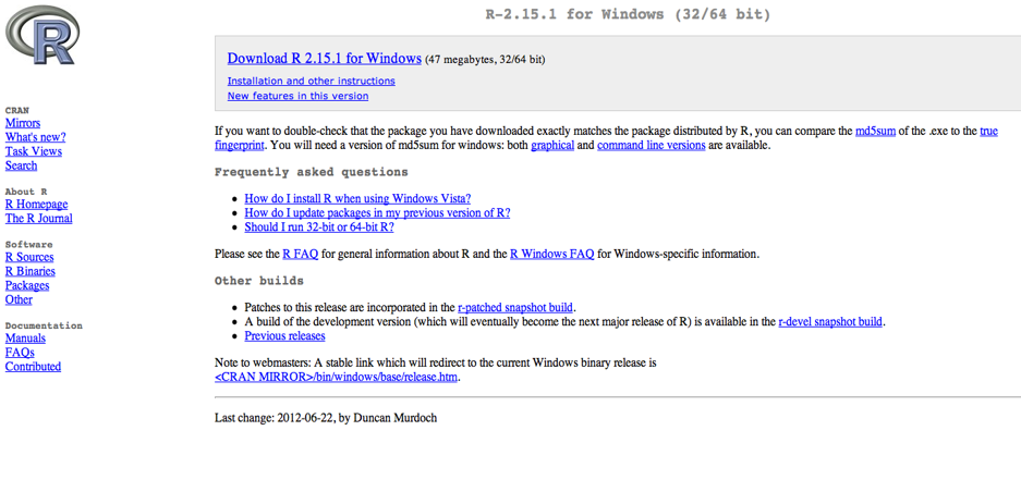
Source: The R project for Statistical Computing.

Follow the prompts to install R.

With R succesfully installed, let’s now install R Studio, an R IDE (Integrated Development Environment).

First, go to: https://www.rstudio.com/products/rstudio/download/

Download the Desktop - Free version.

Selecting the Installer appropriatte for your system.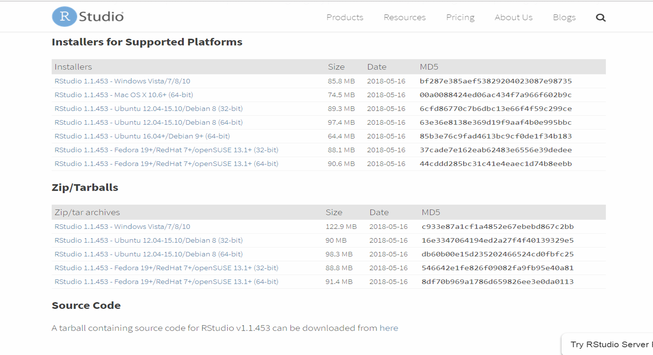

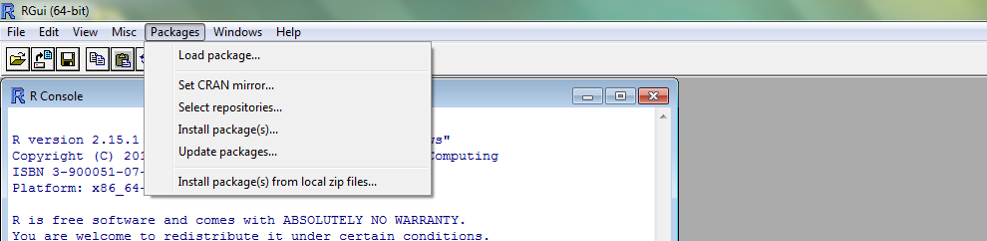
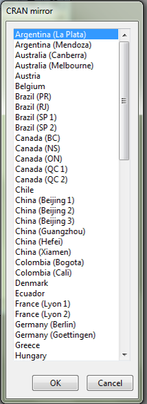
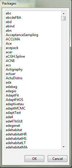
Installing Packages.

11.3 Basics

11.3.1 Operators

Table 11.1: Arithmetic Operators

Operator	Description
+	addition
-	subtraction
*	multiplication
/	division
^ or **	exponentiation
x%%y	modulus (x mod y) 5%%2 is 1
x%/%y	integer division 5%/%2 is 2

Table 11.2: Logical Operators

Operator	Description
<	less than
<=	less than or equal to
>	greater than
>=	greater than or euqal to
==	exactly equal to
!=	not equal to
!x	Not x
x|y	x OR y
x&y	x AND y
isTRUE(x)	test if x is TRUE

11.3.2 Functions

Built-in Functions

• R has many built in functions that compute different statistical procedures.
• Functions in R are followed by ( ).
• Inside the parenthesis we write the object (vector, array, matrix, dataframe) to which we want to apply the function.

Table 11.3: Numeric Functions

Function	Description
abs(x)	absolute value
sqrt(x)	square root
ceiling(x)	ceiling(3.475) is 4
floor(x)	floor(3.475) is 3
trunc(x)	trunc(5.99) is 5
round(x, digits=n)	round(3.475, digits=2) is 3.48
signif(x, digits=n)	signif(3.475, digits=2) is 3.5
cos(x), sin(x), tan(x)	also acos(x), cosh(x), acosh(x), etc.
log(x)	natural logarithm
log10(x)	common logarithm
exp(x)	e^x

Table 11.4: Character Functions

Function	Description
substr(x, start=n1, stop=n2)	Extract or replace substrings in a character vector. x <- “abcdef”, substr(x, 2, 4) is “bcd”
grep(pattern, x, ignore.case=FALSE, fixed=FALSE)	Search for pattern in x. If fixed =FALSE then pattern is a regular expression. If fixed=TRUE then pattern is a text string. Returns matching indices. grep(“A”, c(“b”,“A”,“c”), fixed=TRUE) returns 2
sub(pattern, replacement, x, ignore.case=FALSE, fixed=FALSE)	Find pattern in x and replace with replacement text. If fixed=FALSE then pattern is a regular expression. If fixed = T then pattern is a text string. sub(“”,“.”,“Hello There”) returns “Hello.There”
strsplit(x, split)	Split the elements of character vector x at split. strsplit(“abc”, “”) returns 3 element vector “a”,“b”,“c”
paste(…, sep=“”)	Concatenate strings after using sep string to seperate them. paste(“x”,1:3,sep=“”) returns c(“x1”,“x2” “x3”) paste(“x”,1:3,sep=“M”) returns c(“xM1”,“xM2” “xM3”) paste(“Today is”, date())
toupper(x)	Uppercase
tolower(x)	Lowercase

The following tables describe functions related to probability distributions. For random number generators below, you can use set.seed(1234) or some other integer to create reproducible pseudo-random numbers.

Table 11.5: Statistical / Probability Functions

Function	Description
dnorm(x)	normal density function (by default m=0 sd=1) # plot standard normal curve x <- pretty(c(-3,3), 30) y <- dnorm(x) plot(x, y, type=“l”, xlab=“Normal Deviate”, ylab=“Density”, yaxs=“i”)
pnorm(q)	cumulative normal probability for q (area under the normal curve to the right of q) pnorm(1.96) is 0.975
qnorm(p)	normal quantile. value at the p percentile of normal distribution qnorm(.9) is 1.28 # 90th percentile
rnorm(n, m=0, sd=1)	n random normal deviates with mean m and standard deviation sd. #50 random normal variates with mean=50, sd=10x <- rnorm(50, m=50, sd=10)
dbinom(x, size, prob), pbinom(p, size,prob), qbinom(q,size,prob), rbinom(n,size,prob)	binomial distribution where size is the sample size and prob is the probability of a heads (pi) # prob of 0 to 5 heads of fair coin out of 10 flips dbinom(0:5, 10, .5) # prob of 5 or less heads of fair coin out of 10 flips pbinom(5, 10, .5)
dpois(x, lamda), ppois(q,lamda), qpois(p,lamda), rpois(n,lamda)	poisson distribution with m=std=lamda #probability of 0,1, or 2 events with lamda=4 dpois(0:2, 4) # probability of at least 3 events with lamda=4 1- ppois(2,4)
dunif(x,min,max=1)	uniform distribution, follows the same pattern
punif(q,min=0,max=1)	as the normal distribution above.
qunif(p,min=0,max=1)	#10 uniform random variates
runif(n,min=0,max=1)	x <- runif(10)
mean(x,trim=0, na.rm=FALSE)	mean of object x, # trimmed mean, removing any missing values and # 5 percent of highest and lowest scores mx <- mean(x,trim=.05,na.rm=TRUE)
sd(x)	standard deviation of object(x). also look at var(x) for variance and mad(x) for median absolute deviation.
median(x)	median
quantile(x)	quantiles where x is the numeric vector whose quantiles are desired and probs is a numeric vector with probabilities in [0,1]. # 30th and 84th percentiles of x, y <- quantile(x, c(.3,.84))
range(x)	range
sum(x)	sum
diff(x,lag=1)	lagged differences, with lag indicating which lag to use
min(x)	minimum
max(x)	maximum
scale(x, center=TRUE, scale=TRUE)	column center or standardize a matrix

Table 11.6: Other Functions

Function	Description
seq(from, to, by)	generate a sequence indices <- seq(1,10,2) #indices is c(1, 3, 5, 7, 9)
rep(x,ntimes)	repeat x n times y <- rep(1:3, 2) # y is c(1, 2, 3, 1, 2, 3)
cut(x,n)	divide continuous variable in factor with n levels y <- cut(x, 5)
length(object)	number of elements or components
str(object)	structure of an object
class(object)	class or type of an object
names(object)	names
c(object, object,…)	combine objects into a vector
cbind(object, object,…)	combine objects as columns
rbind(object, object,…)	combine objects as rows
ls()	list current objects
rm(object)	delete an object
newobject <- edit(object)	create a new object
fix(object)	edit an object in place

Functions Applied

R as a Calculator

1250 + 1000

[1] 2250

1250 - 1000

[1] 250

99/3

[1] 33

3^3

[1] 27

4%%2

[1] 0

1+1; 4*5; 6-2

[1] 2 [1] 20 [1] 4

Dealing with NAN and NA’s.

• NAN (not a number)
• NA (missing value)

x <- c(1:8, NA)

####NA is the result
mean(x)

[1] NA

####na.rm removes the NA, so the calculation may be performed
mean(x, na.rm=TRUE)

[1] 4.5

11.3.3 Data Types

String Characters

• In R, string variables are defined by double quotation marks.

letters <- c("A", "B", "C")

Table 11.7: Character String

x
A
B
C

Objects in R

• Objects in R obtain values by assignment.
• This is achieved by the gets arrow, <-, and not the equal sign, =.
• Objects can be of different kinds.
• Vectors, Arrays, Matrices, Subscripts, Dataframes

Vector

• A vector is a sequence of data elements of the same basic type. Members in a vector are officially called components.
• Here is a vector containing three numeric values 2, 3 and 5.

vector <- c(2,3,5)

Table 11.8: Vector

x
2
3
5

Array

Arrays are numeric objects with dimension attributes. The difference between a matrix and an array is that arrays have more than two dimensions. The following example creates an array of two 3x3 matrices each with 3 rows and 3 columns.

Create two vectors of different lengths.

vector1 <- c(5,9,3,7,2)
vector2 <- c(10:17)

Take these vectors as into the array.

result <- array(c(vector1, vector2), dim=c(3,3,2))

Table 11.9: Matrix

V1	V2	V3	V4	V5	V6
5	7	11	14	17	3
9	2	12	15	5	7
3	10	13	16	9	2

Matrix

A matrix is a collection of data elements arranged in a two-dimensional rectangular layout. The following is an example of a matrix with 2 rows and 3 columns.

matrix <- matrix(c(2,4,3,1,5,7), # the data elements
            nrow=2, #number of rows
            ncol = 3, #number of columns
            byrow = TRUE) #fill matrix by rows

Table 11.10: Matrix

2	4	3
1	5	7

Subscript

• Select only one or some of the elements in a vector, a matrix or an array.
• We can do this by using subscripts in square brackets .
  
• In matrices or dataframes the first subscript refers to the row and the second to the column.
  
• R has several ways to subscript (that is, extract specific elements from a vector). The most common way is directly using the square bracket operator:

vector1[4]

[1] 7 In this example, the user has said “give me the fourth element of vector1”.

Here is a similar question: “what are the second and fifth elements of vector1?”

vector1[c(2,5)]

[1] 9 2

Here the c(), of course, constructs the vector (2,5) to be used as the index; then we extract the second and fifth entries of vector1.

Dataframe

A data frame is used for storing data tables. It is a list of vectors of equal length. For example, the following variable df is a data frame containing three vectors n, s, b

n <- c(2,3,5)
s <- c("aa","bb","cc")
b <- c(TRUE, FALSE, TRUE)
df <- data.frame(n,s,b) #df is a dataframe

n	s	b
2	aa	TRUE
3	bb	FALSE
5	cc	TRUE

Let’s create a sample data set, summarize the data and perform some basic manipulations.

####Create a vector
x <- (1:5)
####Summarize the vector
summary <- summary(x)
####Calculate the mean and median and check if they are equal
mean <- mean(x)
median <- median(x)
equal <- mean==median
####Transform to a data frame
df <- as.data.frame(x)
####Add a calculated column
df$New <- df$x/2
####Rename the columns
names(df)[names(df)=="x"] <- "Column1"
names(df)[names(df)=="New"] <- "Column2"

Table 11.11: Dataframe

Column1	Column2
1	0.5
2	1.0
3	1.5
4	2.0
5	2.5

Tips

• R is case-sensitive.
• Comment your code so you remember what it does; comments are preceded with #.
• R scripts are simply text files with a .R extension.
• Use Ctrl + R to submit code.
• Use the Tab key to let R/R Studio finish typing commands for you.
• Use Shift + down arrow to highlight lines or blocks of code.
• In R Studio: Ctrl + 1 and Ctrl + 2 switches between script and console.
• Use up and down arrows to cycle through previous commands in console.
• Don’t be afraid of errors; you won’t break R.
• If you get stuck, Google is your friend.

11.3.4 Loops

For loops

In R a while takes this form, where variable is the name of your iteration variable, and sequence is a vector or list of values:

for (variable in sequence) expression

The expression can be a single R command - or several lines of commands wrapped in curly brackets:

for (variable in sequence) { expression expression expression } Here is a quick trivial example, printing the square root of the integers one to ten:

for (x in c(1:10)) print(sqrt(x))

[1] 1 [1] 1.414214 [1] 1.732051 [1] 2 [1] 2.236068 [1] 2.44949 [1] 2.645751 [1] 2.828427 [1] 3 [1] 3.162278

While loops

In R While takes this form, where condition evaluates to a boolean (True/False) and must be wrapped in ordinary brackets:

while (condition) expression

As with a for loop, expression can be a single R command - or several lines of commands wrapped in curly brackets:

while (condition) { expression expression expression }

We’ll start by using a “while loop” to print out the first few Fibonacci numbers: 0, 1, 1, 2, 3, 5, 8, 13, … where each number is the sum of the previous two numbers. Create a new R script file, and copy this code into it:

a <- 0
b <- 1
print(a)

[1] 0

while (b < 50) {
    print(b)
    temp <- a + b
    a <- b
    b <- temp
}

[1] 1 [1] 1 [1] 2 [1] 3 [1] 5 [1] 8 [1] 13 [1] 21 [1] 34

This next version builds up the answer gradually using a vector, which it prints at the end:

x <- c(0,1)
while (length(x) < 10) {
    position <- length(x)
    new <- x[position] + x[position-1]
    x <- c(x,new)
}
print(x)

To understand how this manages to append the new value to the end of the vector x, try this at the command prompt:

x <- c(1,2,3,4)
c(x,5)

[1] 1 2 3 4 5

Writing Functions

This following script uses the function() command to create a function (based on the code above) which is then stored as an object with the name Fibonacci:

Fibonacci <- function(n) {
    x <- c(0,1)
    while (length(x) < n) {
        position <- length(x)
        new <- x[position] + x[position-1]
        x <- c(x,new)
    }
    return(x)
}

Once you run this code, there will be a new function available which we can now test:

Fibonacci(10)

[1] 0 1 1 2 3 5 8 13 21 34

Fibonacci(3)

[1] 0 1 1

Fibonacci(2)

[1] 0 1

Fibonacci(1)

[1] 0 1

That seems to work nicely - except in the case n == 1 where the function is returning the first two Fibonacci numbers! This gives us an excuse to introduce the if statement.

The If statement In order to fix our function we can do this:

Fibonacci <- function(n) {
    if (n==1) return(0)
    x <- c(0,1)
    while (length(x) < n) {
        position <- length(x)
        new <- x[position] + x[position-1]
        x <- c(x,new)
    }
    return(x)
}

In the above example we are using the simplest possible if statement:

if (condition) expression The if statement can also be used like this:

if (condition) expression else expression And, much like the while and for loops the expression can be multiline with curly brackets:

Fibonacci <- function(n) {
    if (n==1) {
        x <- 0
    } else {
        x <- c(0,1)
        while (length(x) < n) {
            position <- length(x)
            new <- x[position] + x[position-1]
            x <- c(x,new)
        }
    }
    return(x)
}

Fibonacci(1)

[1] 0

11.4 References

’`

1. EMC2, “IDC Digital Universe Study: Big Data, Bigger Digital Shadows and Biggest growth in the Far East. 2011.

2. Beller, Michael J.; Alan Barnett (2009-06-18). “Next Generation Business Analytics”. Lightship Partners LLC. Retrieved 2009-06-20.

3. Wickham, Hadley, and Garrett Grolemund. R For Data Science: Import, Tidy, Transform, Visualize and Model Data. OReilly, 2017.

4. Statmethods.net. (2018). Quick-R: Home Page. [online] Available at: https://www.statmethods.net/ [Accessed 13 Jul. 2018].

5. Wickham, Hadley. Advanced R. CRC Press, 2017.

6. https://warwick.ac.uk/fac/sci/moac/degrees/moac/ch923/r_introduction/r_programming/

7. Schierwagen, Andreas. (2009). Brain Complexity: Analysis, Models and Limits of Understanding. 195-204. 10.1007/978-3-642-02264-7_21.

8. https://josepcurtodiaz.gitbooks.io/customer-analytics-with-r/content/chapter3.html

9. http://r-statistics.co/Linear-Regression.html

10. https://github.com/nicolasfguillaume/Marketing-Analytics-with-R/blob/master/module4.md

11. https://datascienceplus.com/six-sigma-dmaic-series-in-r-part-1/