Chapter 2 New Analysis
2.1 data step 1
library(tidyverse)
library(htmlTable)
library(readxl)
library(ggrepel)
#library(doMC)
#registerDoMC(31)
library(data.table)
library(DT)
library(plotly)
library(readr)
2.2 load data of Int and Kr
data import of international and korea
getwd()## [1] "/home/sehnr/projects/covid_int/occup_health"#new laura data Dec 2020
#korea data
#write_csv(covid_data, '/home/sehnr/projects/covid_int/data/covid.csv')
covid = read_csv('/home/sehnr/projects/covid_int/data/covid.csv')
kr_d <- read_xlsx('data/kr_data.XLSX', sheet = 1)
#international data
cbook <- read_xlsx('data/code_book.xlsx')country_lkup <- data.frame(country = c(1, 16, 31, 36,65, 75, 79, 104, 136, 137, 143, 156, 168, 172, 173, 179, 183, 192),
country_c = c(
"USA", "Belarus", "Canada", "China",
"German", "Hong Kong", "Indonesia",
"Malaysia", "Philipines", "Poland",
"Rusia", "Singapore", "Sweden",
"Thailand", "Taiwan", "Turkey",
"Ukraina", "Vietnam"
))overview of codebook
cbook %>% datatable() 'country' = Q2,
'gender' = Q10,
'Birthyear' = Q79,
'Education' = Q80,
'Employment' = Q94,
'today_dep_anxi' = Q41_5, # for korea 'Q22_5'
'emotion_dpressed' = Q36_2, # for korea Q18_2 : how much...
'emotion_anxiety' = Q36_3, # for Korea Q18_3Korea Data step
kr_d1 <- kr_d %>%
      select('IDnum' = No, 'age' = SQ2, 'gender' = SQ1, 'Education'  = DQ1,
             contains('DQ2'), # employment status
             'EmoDep'  = Q18_2, # for int Q36_2 how much have you feeling
             'EmoAnx'  = Q18_2, # for int Q36_3
             'ChrDep'  = Q21_10, # for int Q40_17
             'ChrAnx'  = Q21_11, # for int Q40_18
             'ToDepAnx'= Q22_5, # for int Q41_5,
             'dfLossJob' = Q10_10, # for int Q26_9,
             'dfReduIcm' = Q10_3, # for int Q26_3,
             'dfIncAnx'  = Q10_5 # for int Q26_5
             ) %>%
  mutate(country = 200, country_c = 'Korea') %>%
  map_if(is.numeric, ~ifelse(is.na(.x), 0, .x) ) %>%
 as.data.frame()

#colnames(kr_d1) <- colnames(kr_d1) %>%
#                       str_replace(., "DQ2_", "em")
colnames(kr_d1)
## [1] "IDnum" "age" "gender" "Education" "DQ2_1" "DQ2_2"
## [7] "DQ2_3" "DQ2_4" "DQ2_5" "DQ2_6" "DQ2_7" "DQ2_8"
## [13] "DQ2_9" "DQ2_10" "DQ2_11" "DQ2_12" "DQ2_13" "DQ2_14"
## [19] "EmoDep" "EmoAnx" "ChrDep" "ChrAnx" "ToDepAnx" "dfLossJob"
## [25] "dfReduIcm" "dfIncAnx" "country" "country_c"international Data step
int_d1 <- covid %>%
      mutate('age' = 2020 - Q79) %>%
     mutate(IDnum = row_number()) %>%
      select(IDnum,
             'age',
             'gender' = Q10, 'Education'  = Q80,
             contains('Q94'), # employment status
             'EmoDep'  = Q36_2,
             'EmoAnx'  = Q36_3,
             'ChrDep'  = Q40_17,
             'ChrAnx'  = Q40_18,
             'ToDepAnx'= Q41_5,
             'dfLossJob' = Q26_9,
             'dfReduIcm' = Q26_3,
             'dfIncAnx'  = Q26_5,
             'country' = Q2
             ) %>%

   left_join(country_lkup,  by = c('country')) %>%
   select(-Q94_18, -Q94_19)
Harmonizing Variable name to int
em_lkup = tibble(
  'kr' = c('DQ2_1', 'DQ2_2', 'DQ2_3', 'DQ2_4', 'DQ2_5', 'DQ2_6', 'DQ2_7',
           'DQ2_8','DQ2_9','DQ2_10','DQ2_11','DQ2_12','DQ2_13','DQ2_14'),
  'int' =c('Q94_9', 'Q94_2',    'Q94_3',    'Q94_4',    'Q94_7',    'Q94_8',    'Q94_5',    'Q94_12',   'Q94_14',   'Q94_15',   'Q94_1',    'Q94_6',    'Q94_16',   'Q94_17')

)

kr_d2<- kr_d1 %>%
plyr::rename(setNames(em_lkup$int, em_lkup$kr)) # change kr vairalbe names to int variabl names.

colnames(kr_d2)   == colnames(int_d1)
## [1] TRUE TRUE TRUE TRUE TRUE TRUE TRUE TRUE TRUE TRUE TRUE TRUE TRUE TRUE TRUE
## [16] TRUE TRUE TRUE TRUE TRUE TRUE TRUE TRUE TRUE TRUE TRUE TRUE TRUE2.3 data merge
mm <- rbind(int_d1, kr_d2)
nrow(mm)
## [1] 19270mm <- mm %>% na.omit(age)
nrow(mm)## [1] 16942data mutate
krtoint = function(x) {
  x = ifelse(x<4, x+4, x)
}
logictozero= function(x){
  x = as.numeric(x != 0)
}
mm1 <-mm %>%
  filter(age >20 & age <65) %>%
  filter(gender %in% c(1, 2))

mm12<- mm1 %>%
  mutate(EmoDep =krtoint(EmoDep),
         EmoAnx =krtoint(EmoAnx),
         ToDepAnx=ifelse(ToDepAnx == 3, 1, 0)) %>%
  select(-c('ChrDep', 'ChrAnx', 'dfLossJob','dfReduIcm','dfIncAnx' ))

mm13 <- mm1 %>%
  select(c('ChrDep', 'ChrAnx', 'dfLossJob','dfReduIcm','dfIncAnx' )) %>%
  lapply(., logictozero) %>%
  data.frame()

mm2 <- cbind(mm12, mm13)


mm3 <- mm2 %>%
  mutate(EcLoss       = ifelse(Q94_3 !=0 | Q94_4!=0, 1, 0)) %>%
  mutate(EcLossUnSafe = ifelse(Q94_4!=0, 1, 0)) %>%
  mutate(agegp = cut(age, breaks = c(-Inf, (5:13)*5, +Inf))) %>%
  mutate(agegp2 = as.numeric(agegp)) %>%
  mutate(genders = ifelse(gender ==1, 'Men', 'Women')) %>%
  mutate(Edugp = factor(Education, levels = c(1, 2, 3, 4, 5, 6),
                        labels = c("Middle or less", "High", "Colleage",
                                   "University", "Graduate Sc", "Doctoral or more"))) %>%
  mutate(EcLossAll = EcLoss + dfLossJob ) %>%
  mutate(TotalDepAnx= as.numeric((as.numeric(EmoDep ==7) + as.numeric(EmoAnx ==7))) !=0)
2.4 Data analysis start
2.4.1 job loss due to covid vary by country
basic static for job loss prevalance across coutnry and genders.
mm3 %>%
  filter(!country %in% c(16, 173)) %>%
  group_by(country_c, genders) %>%
  count(EcLoss) %>%
  mutate(prob = n/sum(n)) %>%
  filter(EcLoss == 1 ) %>%
  ggplot(aes(x = genders, y = prob, fill = genders)) +
  geom_bar(stat = "identity")+
  ylab("job loss due to COVID19")+
  scale_y_continuous(labels = function(x) paste0(x*100, "%"))+
  facet_wrap(country_c ~., nrow = 4)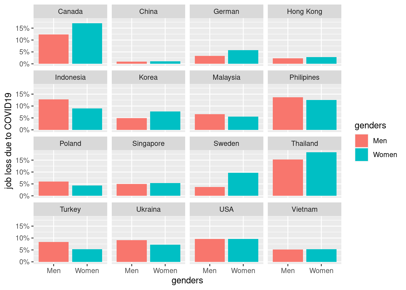
job loss figure (graphical explorer)
mm3 %>%
  filter(!country %in% c(16, 173)) %>%
  group_by(country_c, genders, agegp2) %>%
  count(EcLoss) %>%
  mutate(prob = n/sum(n)) %>%
  filter(EcLoss == 1) %>%
  ggplot(aes(x = agegp2, y = prob, color = genders)) +
  geom_point(aes(size = n), alpha = 0.2, show.legend = FALSE) +
  geom_smooth(method = 'loess', span =0.9,  se=FALSE) +
   ylab("job loss due to COVID19")+
    scale_y_continuous(labels = function(x) paste0(x*100, "%"))+
  theme_minimal() +
  xlab("Age") +
  labs(color = "Gender") +
  facet_wrap(country_c~., nrow =4)
## `geom_smooth()` using formula 'y ~ x'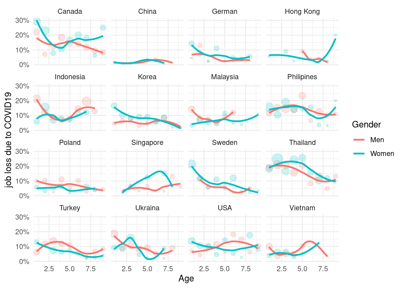
mm3 %>%
  filter(!country %in% c(16, 173)) %>%
  group_by(country_c, genders, agegp2) %>%
  count(dfLossJob) %>%
  mutate(prob = n/sum(n)) %>%
  filter(dfLossJob == 1) %>%
  ggplot(aes(x = agegp2, y = prob, color = genders)) +
  geom_point(aes(size = n), alpha = 0.2, show.legend = FALSE) +
  geom_smooth(method = 'loess', span =0.9,  se=FALSE) +
   ylab("job loss due to COVID19")+
    scale_y_continuous(labels = function(x) paste0(x*100, "%"))+
  theme_minimal() +
  xlab("Age") +
  labs(color = "Gender") +
  facet_wrap(country_c~., nrow =4)
## `geom_smooth()` using formula 'y ~ x'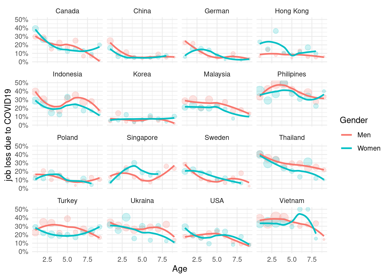
mm3 %>%
  filter(!country %in% c(16, 173)) %>%
  group_by(country_c, genders, agegp2) %>%
  count(dfReduIcm) %>%
  mutate(prob = n/sum(n)) %>%
  filter(dfReduIcm == 1) %>%
  ggplot(aes(x = agegp2, y = prob, color = genders)) +
  geom_point(aes(size = n), alpha = 0.2, show.legend = FALSE) +
  geom_smooth(method = 'loess', span =0.9,  se=FALSE) +
   ylab("dfReduIcm due to COVID19")+
    scale_y_continuous(labels = function(x) paste0(x*100, "%"))+
  theme_minimal() +
  xlab("Age (size = number of respondents)") +
  labs(color = "Gender") +
  facet_wrap(country_c~., nrow =4)
## `geom_smooth()` using formula 'y ~ x'
2.4.2 final job loss status
We decide EcoLossAll as representative valu of job loss.
figure using of EcoLossAll
mm3 %>%
  filter(!country %in% c(16, 173)) %>%
  group_by(country_c, genders, agegp2) %>%
  count(EcLossAll) %>%
  mutate(prob = n/sum(n)) %>%
  filter(EcLossAll == 1) %>%
  ggplot(aes(x = agegp2, y = prob, color = genders)) +
  geom_point(aes(size = n), alpha = 0.2, show.legend = FALSE) +
  geom_smooth(method = 'loess', span =0.9,  se=FALSE) +
   ylab("EcoLossAll due to COVID19")+
    scale_y_continuous(labels = function(x) paste0(x*100, "%"))+
  theme_minimal() +
  xlab("Age (size = number of respondents)") +
  labs(color = "Gender") +
  facet_wrap(country_c~., nrow =4)
## `geom_smooth()` using formula 'y ~ x'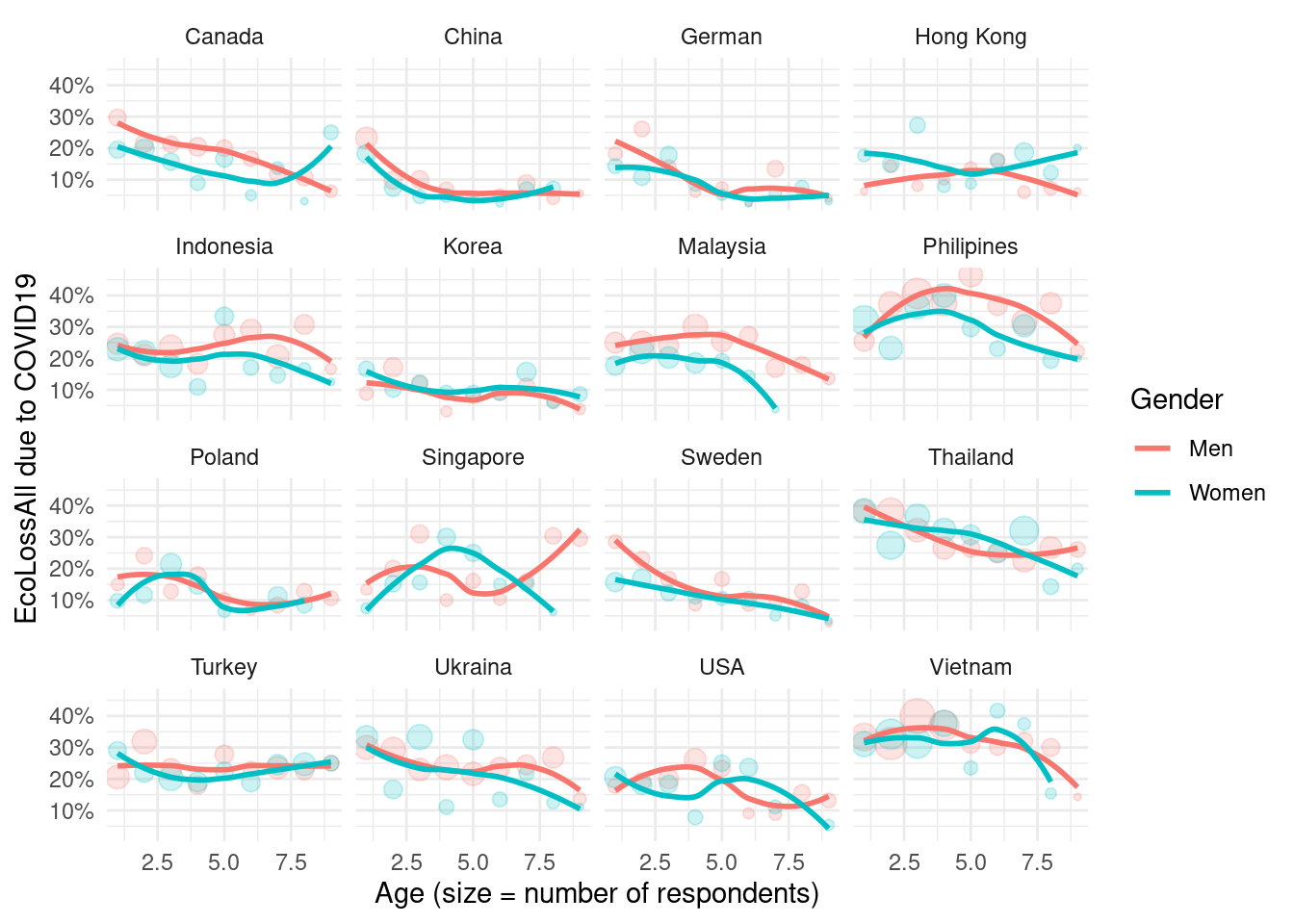
2.4.3 Depression status according job loss status
Depression
mm3 %>%
  filter(!country %in% c(16, 173)) %>%
  group_by(country_c, genders, agegp2) %>%
  count(EmoDep) %>%
  mutate(prob = n/sum(n)) %>%
  filter(EmoDep == 7) %>%
  ggplot(aes(x = agegp2, y = prob, color = genders)) +
  geom_point(aes(size = n), alpha = 0.2, show.legend = FALSE) +
  geom_smooth(method = 'loess', span =0.9,  se=FALSE) +
   ylab("EmoDep due to COVID19")+
    scale_y_continuous(labels = function(x) paste0(x*100, "%"))+
  theme_minimal() +
  xlab("Age") +
  labs(color = "Gender") +
  facet_wrap(country_c~., nrow =4)
## `geom_smooth()` using formula 'y ~ x'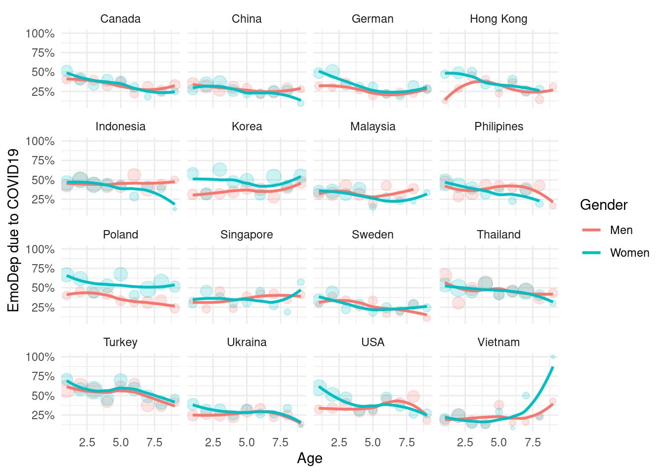
Anxiety
mm3 %>%
  filter(!country %in% c(16, 173)) %>%
  group_by(country_c, genders, agegp2) %>%
  count(EmoAnx) %>%
  mutate(prob = n/sum(n)) %>%
  filter(EmoAnx == 7) %>%
  ggplot(aes(x = agegp2, y = prob, color = genders)) +
  geom_point(aes(size = n), alpha = 0.2, show.legend = FALSE) +
  geom_smooth(method = 'loess', span =0.9,  se=FALSE) +
   ylab("EmoAnx due to COVID19")+
    scale_y_continuous(labels = function(x) paste0(x*100, "%"))+
  theme_minimal() +
  xlab("Age") +
  labs(color = "Gender") +
  facet_wrap(country_c~., nrow =4)
## `geom_smooth()` using formula 'y ~ x'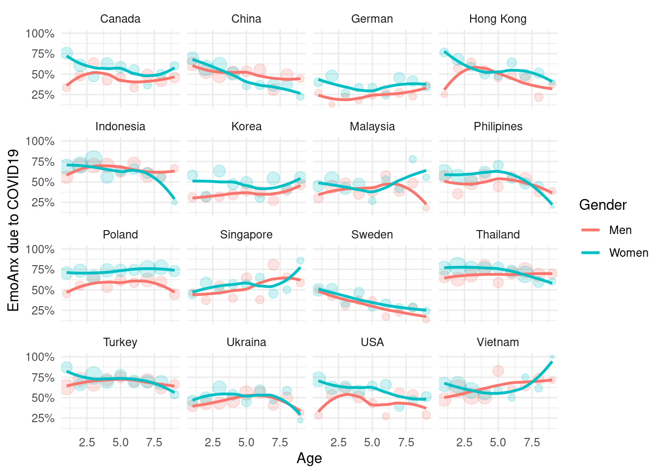
         'EmoDep'  = Q36_2,
         'EmoAnx'  = Q36_3,
         'ChrDep'  = Q40_17,
         'ChrAnx'  = Q40_18,
         'ToDepAnx'= Q41_5,
         'dfLossJob' = Q26_9,
         'dfReduIcm' = Q26_3,
         'dfIncAnx'  = Q26_5,
         'country' = Q2
mm3 %>%
  filter(!country %in% c(16, 173)) %>%
  group_by(country_c, genders, agegp2) %>%
  count(ChrDep) %>%
  mutate(prob = n/sum(n)) %>%
  filter(ChrDep == 1) %>%
  ggplot(aes(x = agegp2, y = prob, color = genders)) +
  geom_point(aes(size = n), alpha = 0.2, show.legend = FALSE) +
  geom_smooth(method = 'loess', span =0.9,  se=FALSE) +
   ylab("ChrDep due to COVID19")+
    scale_y_continuous(labels = function(x) paste0(x*100, "%"))+
  theme_minimal() +
  xlab("Age") +
  labs(color = "Gender") +
  facet_wrap(country_c~., nrow =4)
## `geom_smooth()` using formula 'y ~ x'## Warning in simpleLoess(y, x, w, span, degree = degree, parametric =
## parametric, : pseudoinverse used at 4## Warning in simpleLoess(y, x, w, span, degree = degree, parametric =
## parametric, : neighborhood radius 2## Warning in simpleLoess(y, x, w, span, degree = degree, parametric =
## parametric, : reciprocal condition number 0
mm3 %>%
  filter(!country %in% c(16, 173)) %>%
  group_by(country_c, genders, agegp2) %>%
  count(ChrAnx) %>%
  mutate(prob = n/sum(n)) %>%
  filter(ChrAnx == 1) %>%
  ggplot(aes(x = agegp2, y = prob, color = genders)) +
  geom_point(aes(size = n), alpha = 0.2, show.legend = FALSE) +
  geom_smooth(method = 'loess', span =0.9,  se=FALSE) +
   ylab("ChrAnx due to COVID19")+
    scale_y_continuous(labels = function(x) paste0(x*100, "%"))+
  theme_minimal() +
  xlab("Age") +
  labs(color = "Gender") +
  facet_wrap(country_c~., nrow =4)
## `geom_smooth()` using formula 'y ~ x'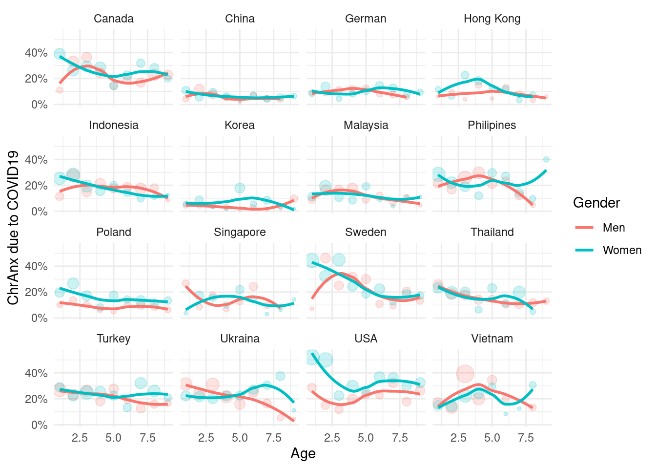
mm3 %>%
  filter(!country %in% c(16, 173)) %>%
  group_by(country_c, genders, agegp2) %>%
  count(ToDepAnx) %>%
  mutate(prob = n/sum(n)) %>%
  filter(ToDepAnx == 1) %>%
  ggplot(aes(x = agegp2, y = prob, color = genders)) +
  geom_point(aes(size = n), alpha = 0.2, show.legend = FALSE) +
  geom_smooth(method = 'loess', span =0.9,  se=FALSE) +
   ylab("ToDepAnx due to COVID19")+
    scale_y_continuous(labels = function(x) paste0(x*100, "%"))+
  theme_minimal() +
  xlab("Age") +
  labs(color = "Gender") +
  facet_wrap(country_c~., nrow =4)
## `geom_smooth()` using formula 'y ~ x'## Warning in simpleLoess(y, x, w, span, degree = degree, parametric =
## parametric, : span too small. fewer data values than degrees of freedom.## Warning in simpleLoess(y, x, w, span, degree = degree, parametric =
## parametric, : pseudoinverse used at 0.965## Warning in simpleLoess(y, x, w, span, degree = degree, parametric =
## parametric, : neighborhood radius 3.035## Warning in simpleLoess(y, x, w, span, degree = degree, parametric =
## parametric, : reciprocal condition number 0## Warning in simpleLoess(y, x, w, span, degree = degree, parametric =
## parametric, : There are other near singularities as well. 36.421## Warning in simpleLoess(y, x, w, span, degree = degree, parametric =
## parametric, : span too small. fewer data values than degrees of freedom.## Warning in simpleLoess(y, x, w, span, degree = degree, parametric =
## parametric, : pseudoinverse used at 5.99## Warning in simpleLoess(y, x, w, span, degree = degree, parametric =
## parametric, : neighborhood radius 1.01## Warning in simpleLoess(y, x, w, span, degree = degree, parametric =
## parametric, : reciprocal condition number 0## Warning in simpleLoess(y, x, w, span, degree = degree, parametric =
## parametric, : There are other near singularities as well. 1.0201## Warning in simpleLoess(y, x, w, span, degree = degree, parametric =
## parametric, : span too small. fewer data values than degrees of freedom.## Warning in simpleLoess(y, x, w, span, degree = degree, parametric =
## parametric, : pseudoinverse used at 0.96## Warning in simpleLoess(y, x, w, span, degree = degree, parametric =
## parametric, : neighborhood radius 3.04## Warning in simpleLoess(y, x, w, span, degree = degree, parametric =
## parametric, : reciprocal condition number 0## Warning in simpleLoess(y, x, w, span, degree = degree, parametric =
## parametric, : There are other near singularities as well. 25.402## Warning in simpleLoess(y, x, w, span, degree = degree, parametric =
## parametric, : span too small. fewer data values than degrees of freedom.## Warning in simpleLoess(y, x, w, span, degree = degree, parametric =
## parametric, : pseudoinverse used at 0.98## Warning in simpleLoess(y, x, w, span, degree = degree, parametric =
## parametric, : neighborhood radius 2.02## Warning in simpleLoess(y, x, w, span, degree = degree, parametric =
## parametric, : reciprocal condition number 0## Warning in simpleLoess(y, x, w, span, degree = degree, parametric =
## parametric, : There are other near singularities as well. 9.1204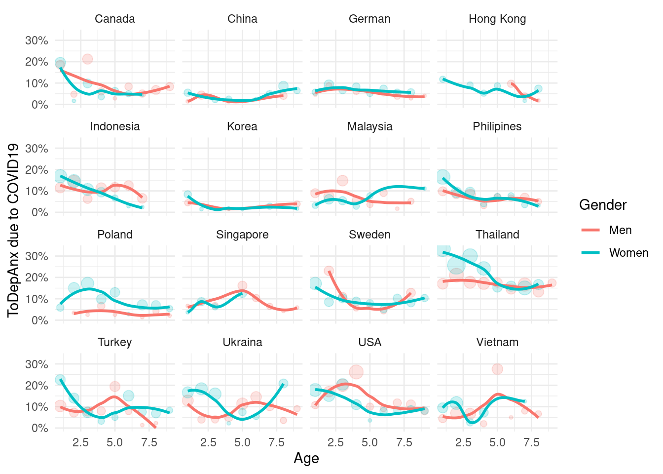
mm3 %>%
  filter(!country %in% c(16, 173)) %>%
  group_by(country_c, genders, agegp2) %>%
  count(TotalDepAnx) %>%
  mutate(prob = n/sum(n)) %>%
  filter(TotalDepAnx == 1) %>%
  ggplot(aes(x = agegp2, y = prob, color = genders)) +
  geom_point(aes(size = n), alpha = 0.2, show.legend = FALSE) +
  geom_smooth(method = 'loess', span =0.9,  se=FALSE) +
   ylab("TotalDepAnx due to COVID19")+
    scale_y_continuous(labels = function(x) paste0(x*100, "%"))+
  theme_minimal() +
  xlab("Age") +
  labs(color = "Gender") +
  facet_wrap(country_c~., nrow =4)
## `geom_smooth()` using formula 'y ~ x'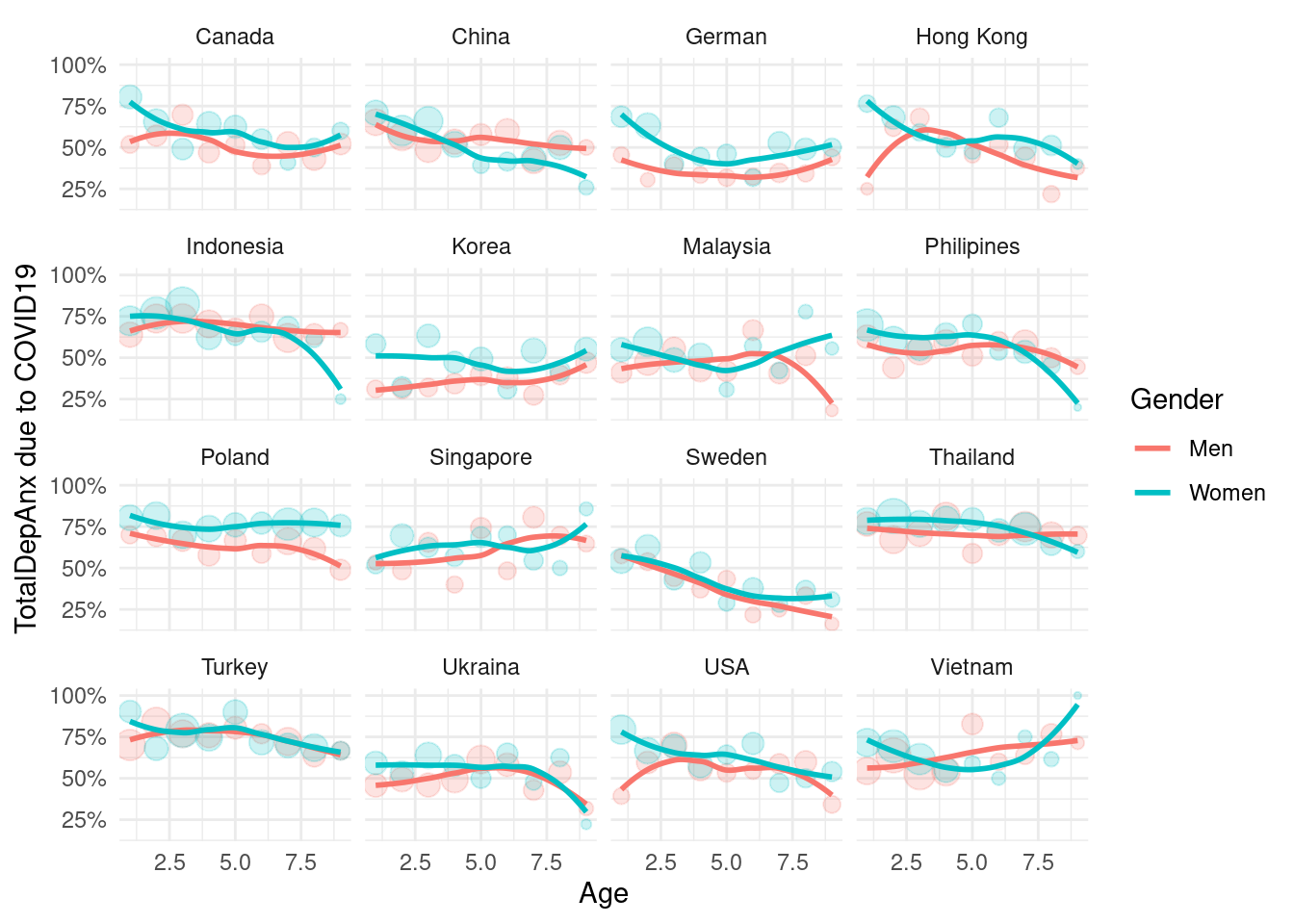
2.5 association
mod1 = mm3 %>%
    glm(family = binomial,
       formula = TotalDepAnx ~ EcLossAll)
mod2 = mm3 %>%
    glm(family = binomial,
formula = TotalDepAnx ~ EcLossAll + age + gender + Education) summary(mod1)$coefficient## Estimate Std. Error z value Pr(>|z|)
## (Intercept) 0.1943074 0.01866925 10.40788 2.282427e-25
## EcLossAll 0.3789140 0.03331761 11.37279 5.713476e-30summary(mod2)$coefficient## Estimate Std. Error z value Pr(>|z|)
## (Intercept) 0.22239927 0.082098954 2.708917 6.750318e-03
## EcLossAll 0.36410397 0.033772468 10.781088 4.228523e-27
## age -0.01075844 0.001393935 -7.718040 1.181323e-14
## gender 0.26873663 0.033879609 7.932105 2.154615e-15
## Education 0.00468844 0.001793254 2.614488 8.936133e-03exp(0.4130821)## [1] 1.511469 mm3 %>%
filter(Education > 0) %>%
group_by(genders, agegp2, Education) %>%
count(TotalDepAnx) %>%
mutate(prob = n/sum(n)) %>%
filter(TotalDepAnx == TRUE) %>%
ggplot(aes(x = agegp2,
y = prob,
color = genders)) +
geom_point() +
geom_smooth() +
facet_wrap(Education~.)## `geom_smooth()` using method = 'loess' and formula 'y ~ x'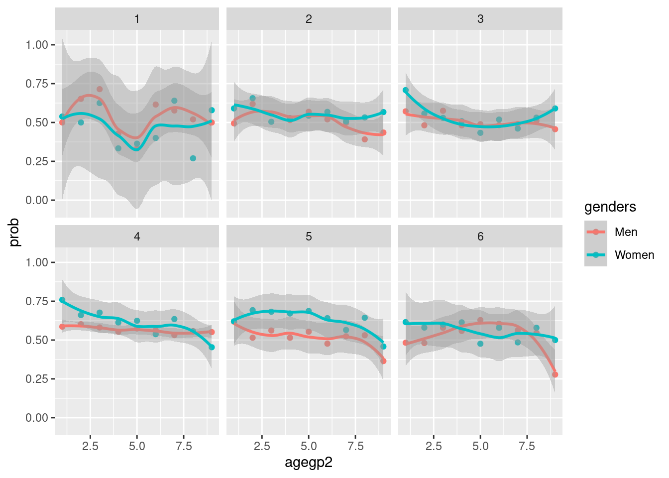
mm4 파일 만들기
mm4 <- mm3 %>%
    mutate(agegp3 = ifelse(age <=40, '≤40', '>40')) %>%
  mutate(agegp3 = factor(agegp3, levels=c('≤40', '>40'))) %>%

  filter(Education %in% c(1:6)) %>%
 mutate(edugp = ifelse(Education %in% c(1, 2), 1,
                        ifelse(Education %in% c(3),2,
                               ifelse(Education %in% c(4), 3, 4)))) %>%
 mutate(edugp2 = ifelse(Education %in% c(1, 2, 3), 1, 2))

bm1<-crossing(
    'genders'=unique(mm4$genders),
    'country_c'=unique(mm4$country_c),
    'edugp'=unique(mm4$edugp),
    'edugp2'=unique(mm4$edugp2),
    'agegp2'=unique(mm4$agegp2),
    'agegp3'=unique(mm4$agegp3),
    'EcLossAll'=unique(mm4$EcLossAll),
    'TotalDepAnx' = unique(mm4$TotalDepAnx)
)
mm4 %>%
group_by(country_c, genders, agegp2) %>%
count(EcLossAll)%>%
full_join(bm1 %>%
select(-edugp, -agegp3, -edugp2) %>%
unique(), by = c('genders', 'country_c', 'agegp2', 'EcLossAll')) %>%
mutate(n = ifelse(is.na(n), 0, n))%>%
mutate(prob = n/sum(n)) %>%
filter(EcLossAll ==1) %>%
ggplot(aes(x = agegp2, y = prob, color = genders, linetype = genders)) +
geom_point(aes(size = n), alpha = 0.2, show.legend = FALSE) +
geom_smooth(method = 'loess', span =1, se=FALSE) +
ylab("job loss due to COVID19")+
labs(color = "Gender", linetype ="Gender") +
scale_x_continuous(breaks = c(1:4*2),
labels = c(15+(1:4)*10)) +
scale_y_continuous(labels = function(x) paste0(x*100, "%"))+
theme_minimal() +
xlab("Age") +
facet_wrap(country_c~., nrow =3)## `geom_smooth()` using formula 'y ~ x'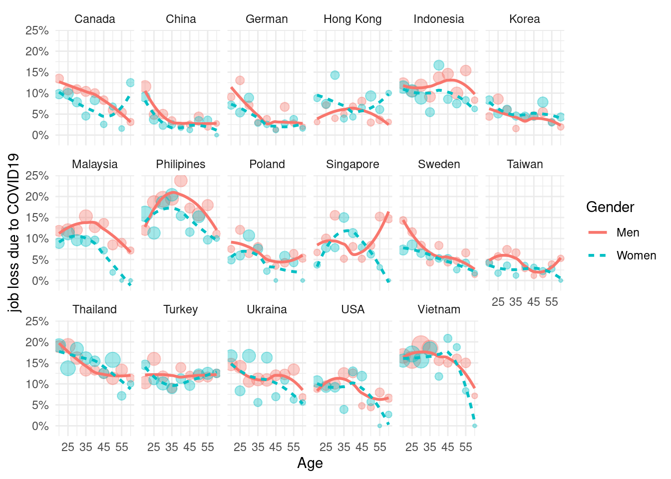
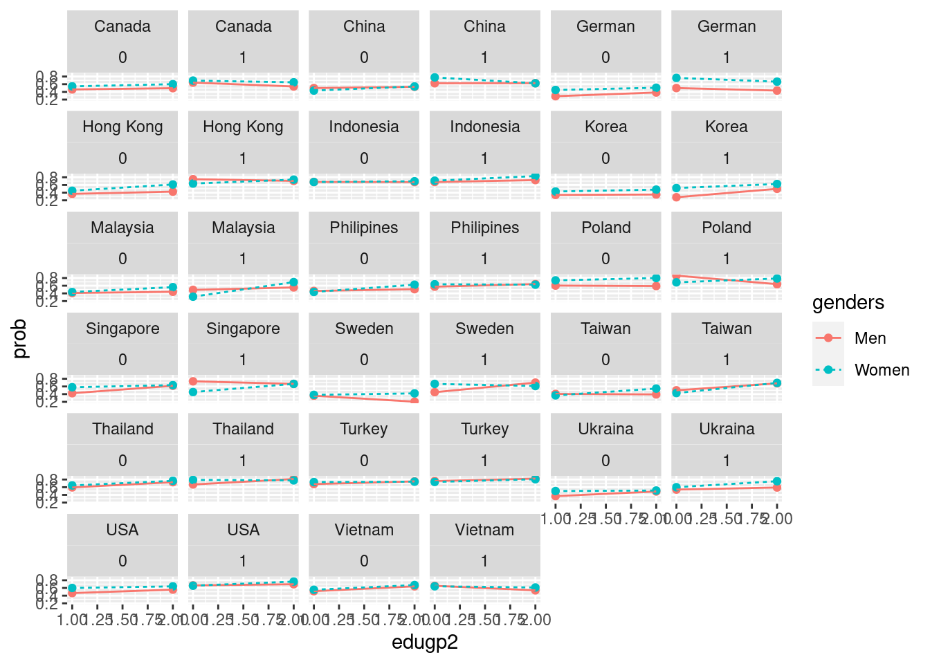
Education
mm4 %>%
  group_by(country_c, genders, edugp2) %>%
  count(EcLossAll)%>%
  full_join(bm1 %>%
              select(-edugp, -agegp3, -agegp2) %>%
              unique(), by = c('genders', 'country_c', 'edugp2', 'EcLossAll')) %>%
  mutate(n = ifelse(is.na(n), 0, n))%>%
  mutate(prob = n/sum(n)) %>%
  filter(EcLossAll ==1) %>%

  ggplot(aes(x = edugp2, y = prob, color = genders, linetype = genders)) +
  #geom_point(aes(size = n), alpha = 0.2, show.legend = FALSE) +
  #geom_smooth(method = 'loess', span =1,  se=FALSE) +
  geom_point()+
  geom_line()+
  ylab("EcLossAll ")+
  labs(color = "Gender", linetype ="Gender") +
  scale_x_continuous(breaks = c(1,  2),
                     labels = c('L',  'H')) +
  scale_y_continuous(labels = function(x) paste0(x*100, "%"))+
  theme_minimal() +
  xlab("Education (< University vs University)") +
  facet_wrap(country_c~., nrow =3)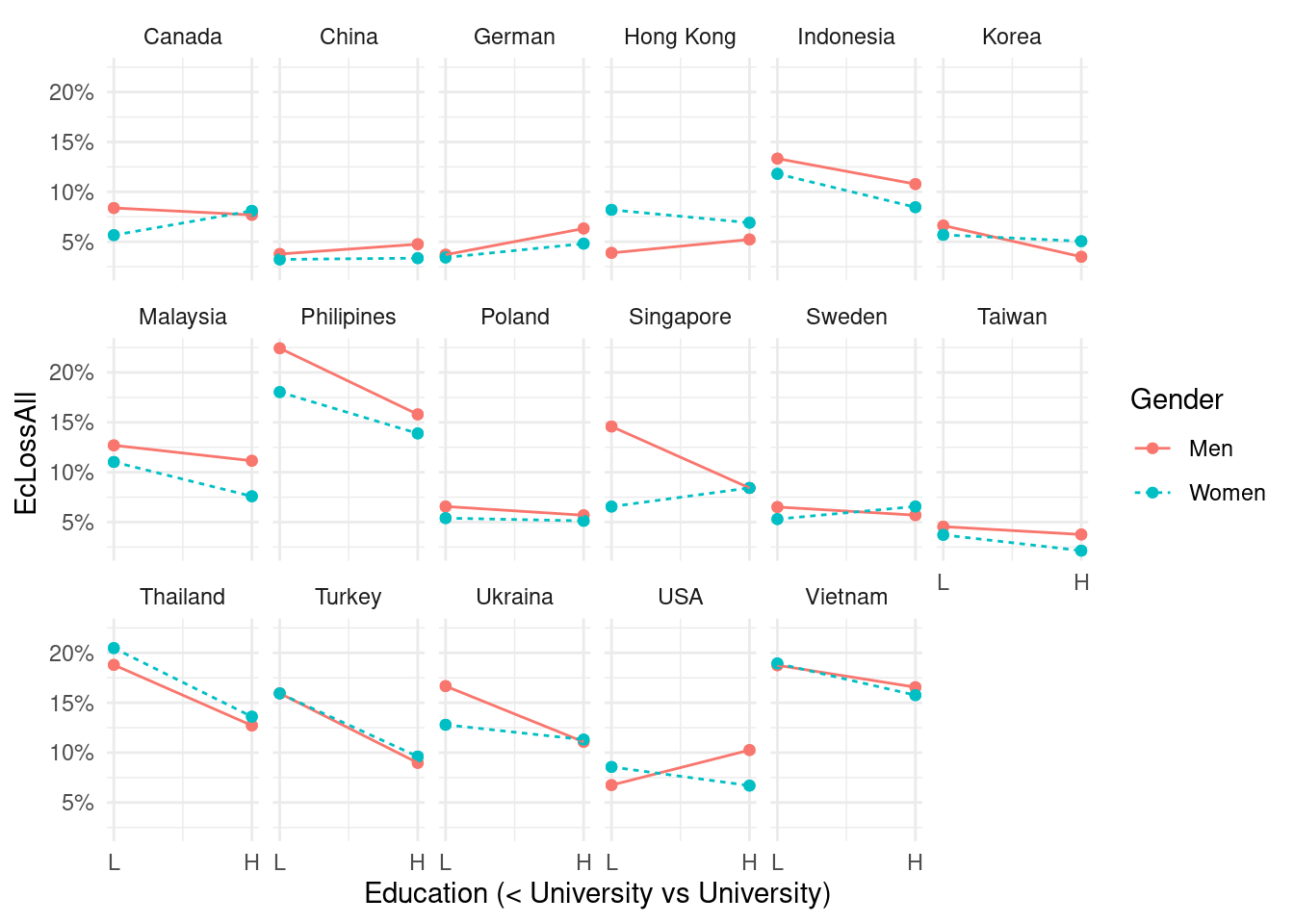
mm4 %>%
  group_by(country_c, genders, edugp2) %>%
  count(TotalDepAnx)%>%
  full_join(bm1 %>%
              select(-edugp, -agegp3, -agegp2) %>%
              unique(), by = c('genders', 'country_c', 'edugp2', 'TotalDepAnx')) %>%
  mutate(n = ifelse(is.na(n), 0, n))%>%
  mutate(prob = n/sum(n)) %>%
  filter(TotalDepAnx == TRUE) %>%

  ggplot(aes(x = edugp2, y = prob, color = genders, linetype = genders)) +
  #geom_point(aes(size = n), alpha = 0.2, show.legend = FALSE) +
  #geom_smooth(method = 'loess', span =1,  se=FALSE) +
  geom_point()+
  geom_line()+
  ylab("TotalDepAnx ")+
  labs(color = "Gender", linetype ="Gender") +
  scale_x_continuous(breaks = c(1,  2),
                     labels = c('L',  'H')) +
  scale_y_continuous(labels = function(x) paste0(x*100, "%"))+
  theme_minimal() +
  xlab("Education (< University vs University)") +
  facet_wrap(country_c~., nrow =3)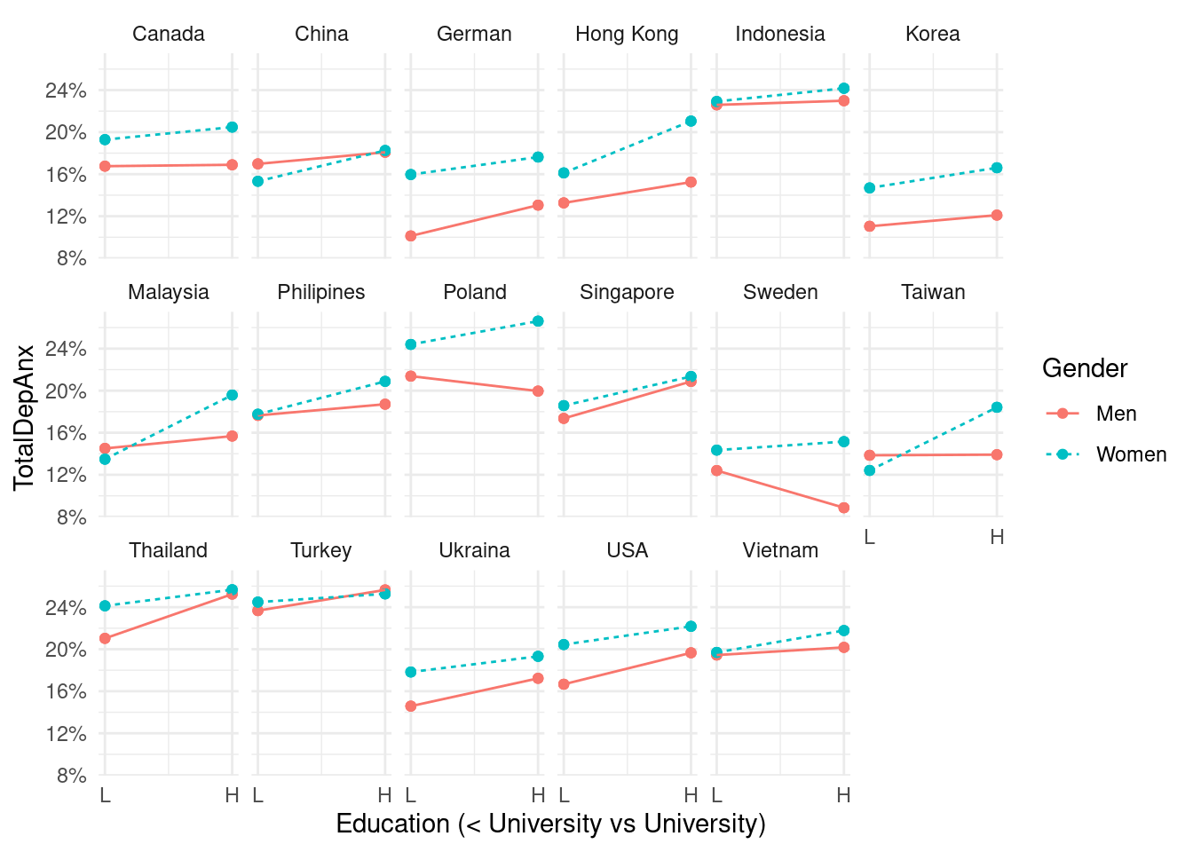
agu1 <- read_csv('data/covid_agu1.csv')## Parsed with column specification:
## cols(
## country_c = col_character(),
## c_case_agu1 = col_double(),
## c_death_agu1 = col_double(),
## population = col_double()
## )mm5 <- mm4 %>%
left_join(agu1, by = 'country_c') %>%
mutate(inc_aug = c_case_agu1 / population *100000,
dth_aug = c_death_agu1/ population *100000)
lab_mm <- mm5 %>%
group_by(country_c, genders) %>%
summarize (edu = mean(edugp),
ecl = mean(EcLossAll !=0),
inc = mean(inc_aug))## `summarise()` has grouped output by 'country_c'. You can override using the `.groups` argument.lab_mm2 <- mm5 %>%
group_by(country_c, genders, agegp3) %>%
summarize(edu = mean(edugp),
ecl = mean(EcLossAll !=0),
inc = mean(inc_aug)) ## `summarise()` has grouped output by 'country_c', 'genders'. You can override using the `.groups` argument.lab_mm %>%
ggplot(aes(x = edu, y = ecl, color = inc)) +
geom_point() +
theme_classic()+
xlab("mean education level") +
ylab("prevalance of economic loss") +
ylim(c(-0.1, 0.5)) +xlim(c(2, 4)) +
geom_label_repel(aes(label = country_c),
fill = NA, # 투명하게 해서 겹쳐도 보이게
alpha =1, size = 3, # 작게
box.padding = 0.4, # 분별해서
segment.size =0.1, # 선
force = 2) + # 이것은 무엇일까요?
theme(legend.position="bottom") + theme_minimal() +
geom_smooth(method = 'lm', formula = y ~ poly(x,2), se=FALSE) +
facet_wrap(genders~.)## Warning: Removed 2 rows containing non-finite values (stat_smooth).## Warning: Removed 2 rows containing missing values (geom_point).## Warning: Removed 2 rows containing missing values (geom_label_repel).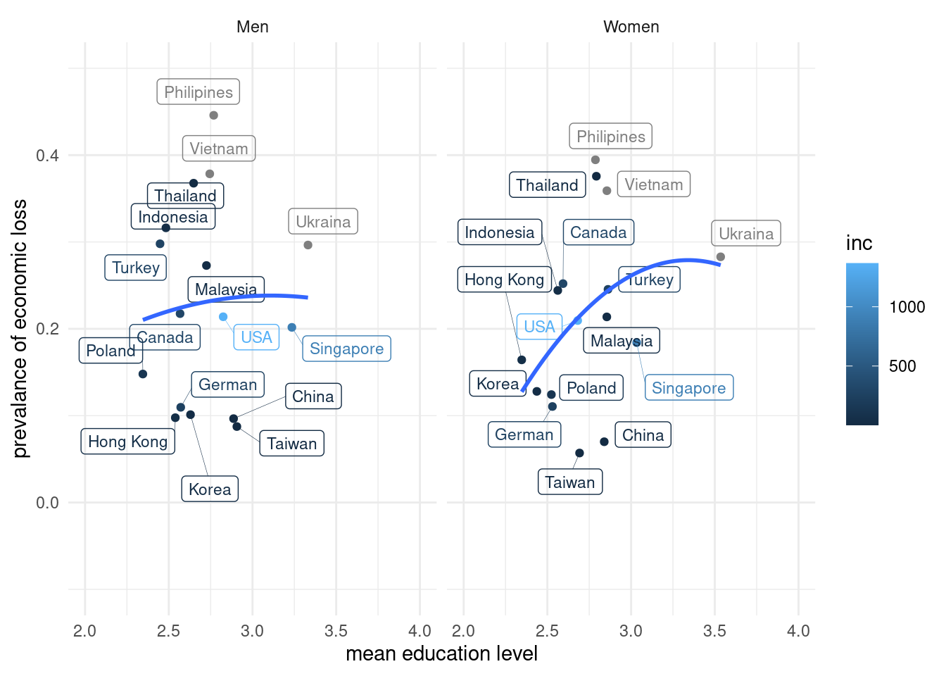
40세
lab_mm2 %>%
  ggplot(aes(x = edu, y = ecl, color = inc)) +
  geom_point() +
  theme_classic()+
  xlab("mean education level") +
  ylab("prevalance of economic loss") +
  ylim(c(-0.1, 0.5)) +xlim(c(2, 4)) +
  geom_label_repel(aes(label = country_c),
                   fill = NA, # 투명하게 해서 겹쳐도 보이게
                   alpha =1, size = 3, # 작게
                   box.padding = 0.4,  # 분별해서
                   segment.size =0.1,  # 선
                   force = 2)      +    # 이것은 무엇일까요?
  theme(legend.position="bottom") + theme_minimal() +
  geom_smooth(method = 'lm', formula = y ~ poly(x,2), se=FALSE) +
  facet_wrap(genders + agegp3~., nrow = 1) +
  scale_x_continuous(breaks = c(2.1, 3, 3.9),
  label = c("high school", "college", ">4y college")
) +
theme(axis.text.x = element_text(angle = -70))
## Scale for 'x' is already present. Adding another scale for 'x', which will
## replace the existing scale.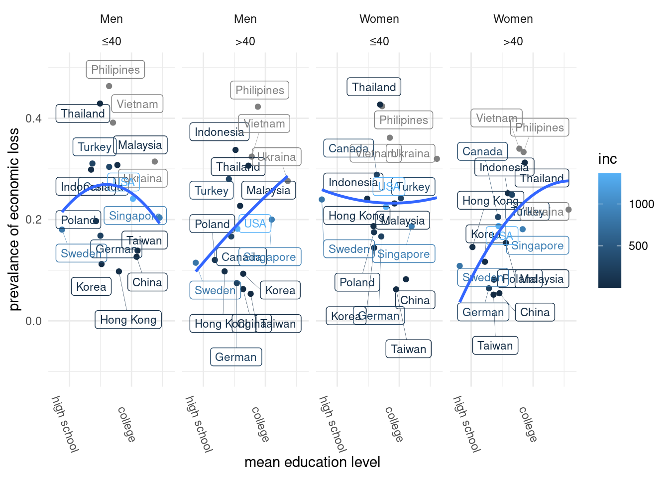
mm5 %>%
  mutate(EcLossAllgp = as.numeric(EcLossAll !=0)) %>%
  group_by(country_c, genders, edugp2, EcLossAllgp) %>%
  count(TotalDepAnx) %>%
  mutate(prob = n/sum(n)) %>%
  filter(TotalDepAnx == TRUE) %>%
  ggplot(aes(x= edugp2, y = prob, color = genders, linetype= genders)) +
  #geom_bar(stat = 'identity') +
  geom_point() + geom_line()+

  facet_wrap(country_c + EcLossAllgp ~.)