Comparing Social Dynamics of a Rental and Purchased Block
Jolene Quek
2018-12-13
1 Observation Mapping
library(tidyverse)
library(dplyr)
library(lubridate)
library(googlesheets4)
library(stringr)
library(ggthemes)
library(plotly)
library(formattable)
library(kableExtra)
1.1 Data cleaning
rental_observations <- read_sheet("1UTywunaRJZyDVXcuXQvy_pNbp1gOgq4GhY9Xpt2SvSI", sheet="blk 499C void deck") ## Reading from 'Observation Mapping'## Range "'blk 499C void deck'"purchased_observations <- read_sheet("1UTywunaRJZyDVXcuXQvy_pNbp1gOgq4GhY9Xpt2SvSI", sheet="blk 485B void deck")## Reading from 'Observation Mapping'## Range "'blk 485B void deck'"# adding column rental or purchased
rental_observations <- rental_observations %>%
mutate(block="rental")
purchased_observations <- purchased_observations %>%
mutate(block="purchased")
# combine the two datasets (rental and purchased)
observations <- rbind(rental_observations, purchased_observations)
# removing the two initial datasets
rm(rental_observations)
rm(purchased_observations)
# renaming and removing columns
observations <- observations %>%
filter(time_in!="NA") %>%
filter(time_out!="NA") %>%
rename(grid='grid (1/2)',
majority_in_same_grid='msg/mnsg',
observer='Observer',
verbal_or_non_verbal='verbal',
planned_or_spontaneous='spontaneous/planned',
remarks='Remarks') %>%
select(-c("duration","description"))
# creating datetime column
observations <- observations %>%
mutate(time_in=sprintf("%04d", time_in)) %>%
mutate(time_out=sprintf("%04d", time_out)) %>%
mutate(hour_in = str_sub(time_in, 1, 2)) %>%
mutate(hour_out = str_sub(time_out, 1, 2)) %>%
mutate(min_in = str_sub(time_in, 3, 4)) %>%
mutate(min_out = str_sub(time_out, 3, 4)) %>%
mutate(seconds = "00") %>%
mutate(time_in = paste0(hour_in, ":", min_in, ":", seconds)) %>%
mutate(time_out = paste0(hour_out, ":", min_out, ":", seconds)) %>%
mutate(date_time_in=paste(date, time_in)) %>%
mutate(date_time_out=paste(date, time_out)) %>%
mutate(date_time_in=as_datetime(date_time_in)) %>%
mutate(date_time_out=as_datetime(date_time_out)) %>%
select(-c("time_in","time_out","date","hour_in","hour_out","min_in","min_out","seconds"))
# cleaning up ethnicity column
observations <- observations %>%
mutate(ethnicity=str_replace_na(ethnicity, replacement = "NA")) %>%
mutate(ethnicity = str_replace(ethnicity,"NA","Unsure")) %>%
mutate(ethnicity = str_replace(ethnicity,"Unknown","Unsure"))
# replace all blanks which appear as NA with "NA"
observations <- observations %>%
replace(., is.na(.), "NA")
# adding id column
observations <- observations %>%
rownames_to_column("id")
# splitting grid column that has multiple responses variables into columns of separate dummy variables
observations <- observations %>%
separate_rows(grid,sep=",") %>% # split a column and append it into the dataset
group_by(id) %>% # shows the mode column and the id column
dplyr::count(grid) %>%
spread(grid, n, fill=0) %>% # shows the matrix of mode by id
dplyr::rename_at(2:4, funs(paste0("grid_", .))) %>% #dplyr::rename columns by adding transport. in front of each mode as a column name
right_join(observations) #join with data## Joining, by = "id"# recode age group column
observations <- observations %>%
mutate(age_group = recode(age_group,
"Below 7"="below 7",
"7-20"="7 to 20",
"20-30"="20 to 30",
"30-40"="30 to 40",
"40-50"="40 to 50",
"50-60"="50 to 65",
"50-65"="50 to 65",
"60-70"="65 to 80",
"65-70"="65 to 80",
"70-80"="65 to 80",
"65-80"="65 to 80"))
# factor and order age_group column
age_group_levels <- c("below 7","7 to 20","20 to 30","30 to 40","40 to 50","50 to 65","65 to 80","above 80")
observations <- observations %>%
mutate(age_group=parse_factor(age_group,levels=age_group_levels,ordered=T))
# typos for gender
observations <- observations %>%
mutate(gender=recode(gender,
"f"="F"))
# recode NA to 1 for group size
observations <- observations %>%
mutate(group_size=recode(group_size,
"NA"="1"))
# adding duration of observation column
observations <- observations %>%
mutate(duration=as.numeric(date_time_out - date_time_in, "mins")) %>%
mutate(duration=recode(duration,
"0"=1)) # for those where date_time_in is the same as date_time_out, we make the duration 1 minute
# recode msg and mnsg
observations <- observations %>%
mutate(majority_in_same_grid=recode(majority_in_same_grid,
"msg"="Y",
"mnsg"="N"))# saving the clean data
rental_observations <- observations %>%
filter(block=="rental")
rental_observations <- apply(rental_observations,2,as.character)
#write.csv(rental_observations,"data/rental_observations.csv")
purchased_observations <- observations %>%
filter(block=="purchased")
purchased_observations <- apply(purchased_observations,2,as.character)
#write.csv(purchased_observations,"data/purchased_observations.csv")A preview of the data we collected during the observation mappings:
library(kableExtra)
kableExtra::kable(head(observations)) %>%
scroll_box(width = "100%", height = "200px")| id | grid_1 | grid_2 | grid_3 | grid | group_size | interacting | planned_or_spontaneous | majority_in_same_grid | verbal_or_non_verbal | gender | age_group | ethnicity | remarks | observer | block | date_time_in | date_time_out | duration |
|---|---|---|---|---|---|---|---|---|---|---|---|---|---|---|---|---|---|---|
| 1 | 1 | 0 | 0 | 1 | 1 | N | NA | NA | NA | M | 50 to 65 | Chinese | NA | Aizat | rental | 1541932860 | 1541932860 | 1 |
| 2 | 1 | 0 | 0 | 1 | 1 | N | NA | NA | NA | M | 20 to 30 | Indian | Cleaner | Aizat | rental | 1541933100 | 1541933160 | 1 |
| 3 | 0 | 0 | 1 | 3 | 1 | N | NA | NA | NA | F | 40 to 50 | Chinese | NA | Aizat | rental | 1541933400 | 1541933400 | 1 |
| 4 | 1 | 0 | 0 | 1 | 1 | N | NA | NA | NA | M | 40 to 50 | Malay | NA | Aizat | rental | 1541933520 | 1541933520 | 1 |
| 5 | 1 | 0 | 0 | 1 | 1 | N | NA | NA | NA | M | 20 to 30 | Chinese | NA | Aizat | rental | 1541933580 | 1541933580 | 1 |
| 6 | 1 | 0 | 0 | 1 | 1 | N | NA | NA | NA | M | 50 to 65 | Malay | NA | Aizat | rental | 1541933700 | 1541933700 | 1 |
1.2 Categorisation of interactions by intensity
Here, we apply the criterion of our rule-based classification.
observations <- observations %>%
  mutate(duration_intensity= case_when(
    duration > 1 ~ "high",
    duration <= 1 ~ "low")) %>%
   mutate(majority_in_same_grid_intensity= case_when(
    majority_in_same_grid == "Y" ~ "high",
    majority_in_same_grid == "N" ~ "low")) %>%
  mutate(verbal_or_non_verbal_intensity= case_when(
    verbal_or_non_verbal == "verbal" ~ "high",
    verbal_or_non_verbal == "non-verbal" ~ "low"))


# categorising intensity of observations
observations <- observations %>%
  mutate(interaction_intensity = case_when(
    duration_intensity == "high" & majority_in_same_grid_intensity == "high" & verbal_or_non_verbal_intensity == "high" ~ "high",
    duration_intensity == "high" & majority_in_same_grid_intensity == "high" & verbal_or_non_verbal_intensity == "low" ~ "high",
    duration_intensity == "high" & majority_in_same_grid_intensity == "low" & verbal_or_non_verbal_intensity == "low" ~ "low",
    duration_intensity == "high" & majority_in_same_grid_intensity == "low" & verbal_or_non_verbal_intensity == "high" ~ "high",
    duration_intensity == "low" & majority_in_same_grid_intensity == "high" & verbal_or_non_verbal_intensity == "low" ~ "low",
    duration_intensity == "low" & majority_in_same_grid_intensity == "high" & verbal_or_non_verbal_intensity == "high" ~ "high",
    duration_intensity == "low" & majority_in_same_grid_intensity == "low" & verbal_or_non_verbal_intensity == "low" ~ "low",
    duration_intensity == "low" & majority_in_same_grid_intensity == "low" & verbal_or_non_verbal_intensity == "high" ~ "low"
  ))

# replace all blanks which appear as NA with "NA", some NAs are introduced for non-interactions in the intensity column
observations <- observations %>%
  replace(., is.na(.), "NA")

# recode NA to "zero" in intensity column for non-interactions
observations<- observations %>%
  mutate(interaction_intensity = recode(interaction_intensity,
                                        "NA"="zero")) %>%
  mutate(duration_intensity = recode(duration_intensity,
                                        "NA"="zero")) %>%
  mutate(majority_in_same_grid_intensity = recode(majority_in_same_grid_intensity,
                                        "NA"="zero")) %>%
  mutate(verbal_or_non_verbal_intensity = recode(verbal_or_non_verbal_intensity,
                                        "NA"="zero"))

# factor and order intensity of interactions
interaction_intensity_levels <- c("zero","low","high")
observations <- observations %>%
  mutate(interaction_intensity=parse_factor(interaction_intensity,levels=interaction_intensity_levels,ordered=T))
1.3 Number of observations per hour by block
observations %>%
  mutate(hour=hour(date_time_in)) %>%
  group_by(block) %>%
  mutate(total_block = n()) %>%
  group_by(hour, block) %>%
  mutate(perc_label = paste(round(n()/total_block*100,1),"%")) %>%
  mutate(perc = n()/total_block*100) %>%
  ggplot(aes(as.factor(hour)))+
  geom_bar(aes(y = perc),stat="identity",position="dodge")+
  geom_text(aes(y=perc,label=perc_label),position=position_dodge(width=0.9),vjust=-0.5, hjust=0.43,size=3,color="black")+
  theme_fivethirtyeight() +
  labs(title="How many observations were \n collected in each hour of a day?\n[observation]") +
  theme(plot.title = element_text(size=14, hjust=0.5))+
  theme(axis.title = element_text()) + xlab('') + ylab('percentage') +
  scale_x_discrete(breaks=c("9","10","11","12","13","14","15","16","17","18","19"),
        labels=c("09:00","10:00","11:00","12:00","13:00","14:00","15:00","16:00","17:00","18:00","19:00"))+
  facet_wrap(block~.)+
  aes(fill = block)+
  theme(panel.spacing = unit(3, "lines"))+
  theme(axis.text.x = element_text(angle = 90, hjust = 1, vjust = 0.5))+
  theme(axis.title.y=element_blank(),
        axis.text.y=element_blank(),
axis.ticks.y=element_blank()) 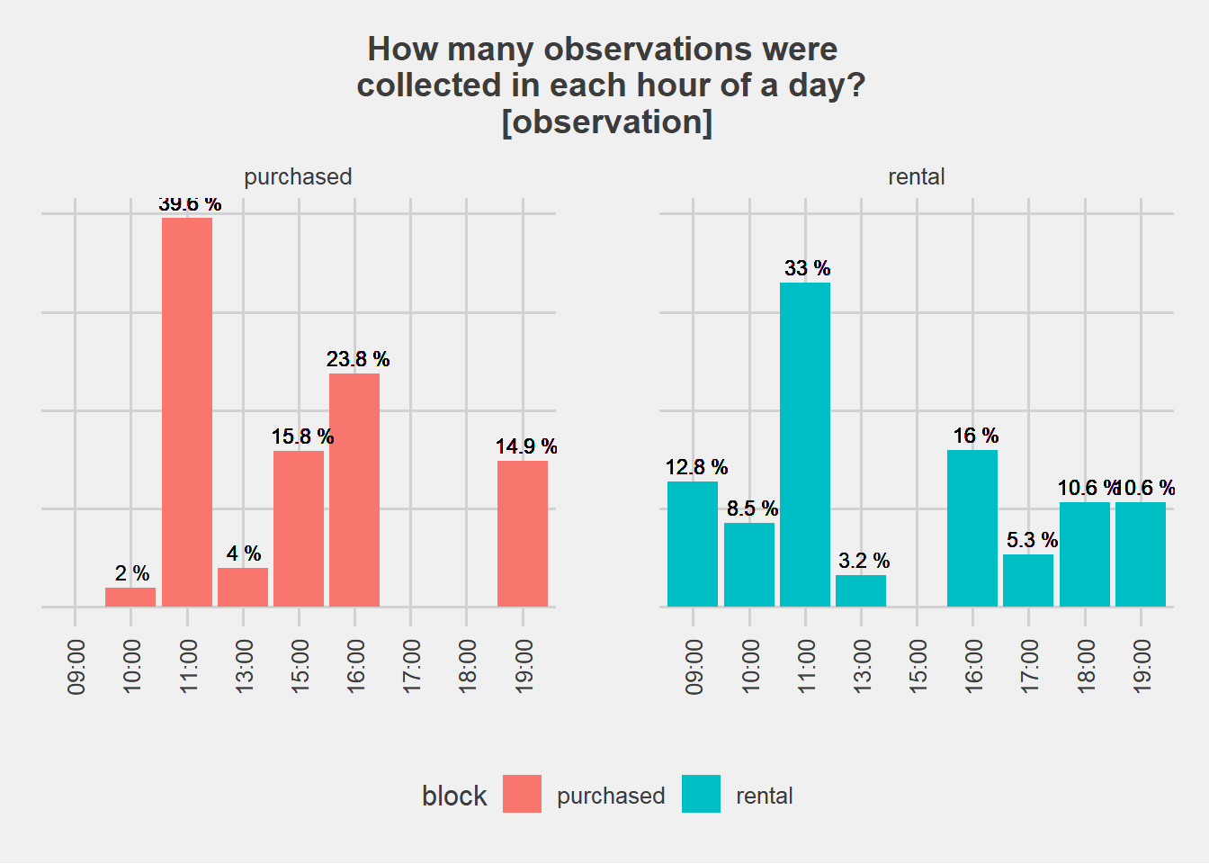
#ggsave("plots/hourly_count.png")1.4 Ethnicities by block
observations %>%
  group_by(block) %>%
  mutate(total_block = n()) %>%
  group_by(ethnicity,block) %>%
  mutate(perc_label = paste(round(n()/total_block*100,1),"%")) %>%
  mutate(perc = n()/total_block*100) %>%
  ggplot(aes((ethnicity), fill=block))+
  geom_bar(aes(y = perc),stat="identity",position="dodge")+
  geom_text(aes(y=perc,label=perc_label),position=position_dodge(width=0.9),vjust=-0.5, hjust=0.43,size=3,color="black")+
  theme_fivethirtyeight() +
  labs(title="Ethnicity by block   [observation]") +
  theme(plot.title = element_text(size=14, hjust=0.5))+
  theme(axis.title = element_text()) + xlab('') + ylab('percentage')+
  theme(axis.title.y=element_blank(),
        axis.text.y=element_blank(),
axis.ticks.y=element_blank()) 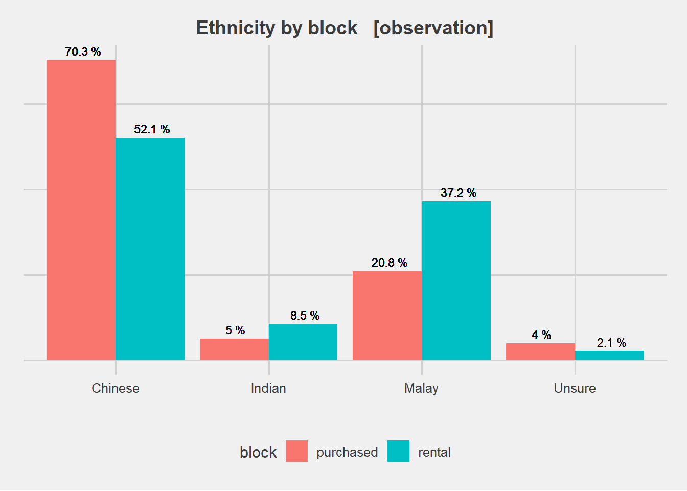
#ggsave("plots/ethnicity.png")1.5 Age-group by block
observations %>%
  filter(age_group!="NA") %>%
  group_by(block) %>%
  mutate(total_block = n()) %>%
  group_by(age_group,block) %>%
  mutate(perc_label = paste(round(n()/total_block*100,1),"%")) %>%
  mutate(perc = n()/total_block*100) %>%
  ggplot(aes(factor(age_group), fill=block))+
  geom_bar(aes(y = perc),stat="identity",position="dodge")+
  geom_text(aes(y=perc,label=perc_label),position=position_dodge(width=0.9),vjust=-0.5, hjust=0.43,size=3,color="black")+
  theme_fivethirtyeight() +
  labs(title="Age groups by block   [observation]") +
  theme(plot.title = element_text(size=14, hjust=0.5))+
  theme(axis.title = element_text()) + xlab('') + ylab('percentage')+
  facet_wrap(block~.)+
  aes(fill = block)+
  theme(panel.spacing = unit(3, "lines"))+
  theme(axis.text.x = element_text(angle = 90, hjust = 1, vjust = 0.5))+
  theme(axis.title.y=element_blank(),
        axis.text.y=element_blank(),
axis.ticks.y=element_blank()) 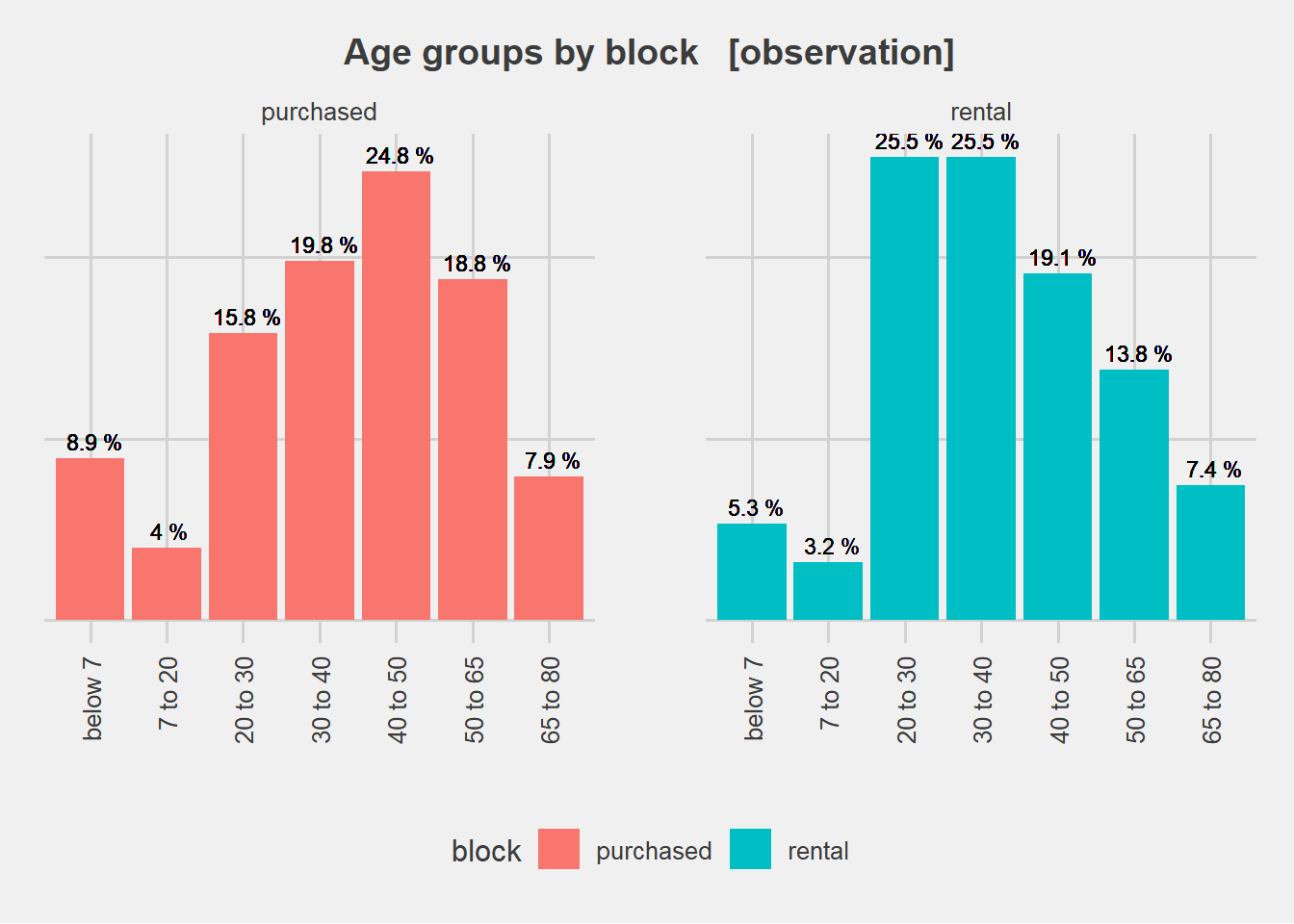
#ggsave("plots/age_group.png")1.6 Gender by block
observations %>%
  filter(gender!="NA") %>%
  filter(gender!="Unsure") %>%
  group_by(block) %>%
  mutate(total_block = n()) %>%
  group_by(gender,block) %>%
  mutate(perc_label = paste(round(n()/total_block*100,1),"%")) %>%
  mutate(perc = n()/total_block*100) %>%
  ggplot(aes((gender), fill=block))+
  geom_bar(aes(y = perc),stat="identity",position="dodge")+
  geom_text(aes(y=perc,label=perc_label),position=position_dodge(width=0.9),vjust=-0.5, hjust=0.43,size=3,color="black")+
  theme_fivethirtyeight() +
  labs(title="Gender by block   [observation]") +
  theme(plot.title = element_text(size=14, hjust=0.5))+
  theme(axis.title = element_text()) + xlab('') + ylab('percentage')+
  scale_x_discrete(breaks=c("F","M"),
        labels=c("Female","Male"))+
  theme(axis.title.y=element_blank(),
        axis.text.y=element_blank(),
axis.ticks.y=element_blank()) 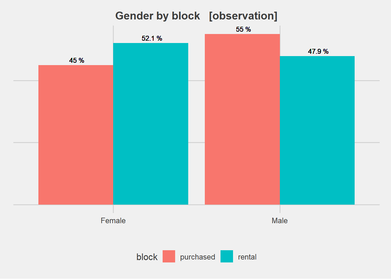
#ggsave("plots/gender.png")1.7 Interaction by block
observations %>%
  group_by(block) %>%
  mutate(total_block = n()) %>%
  group_by(interacting,block) %>%
  mutate(perc_label = paste(round(n()/total_block*100,1),"%")) %>%
  mutate(perc = n()/total_block*100) %>%
  ggplot(aes((interacting), fill=block))+
  geom_bar(aes(y = perc),stat="identity",position="dodge")+
  geom_text(aes(y=perc,label=perc_label),position=position_dodge(width=0.9),vjust=-0.5, hjust=0.43,size=3,color="black")+
  theme_fivethirtyeight() +
  labs(title="Interaction by block   [observation]") +
  theme(plot.title = element_text(size=14, hjust=0.5))+
  theme(axis.title = element_text()) + xlab('') + ylab('percentage')+
  theme(axis.title.y=element_blank(),
        axis.text.y=element_blank(),
axis.ticks.y=element_blank()) 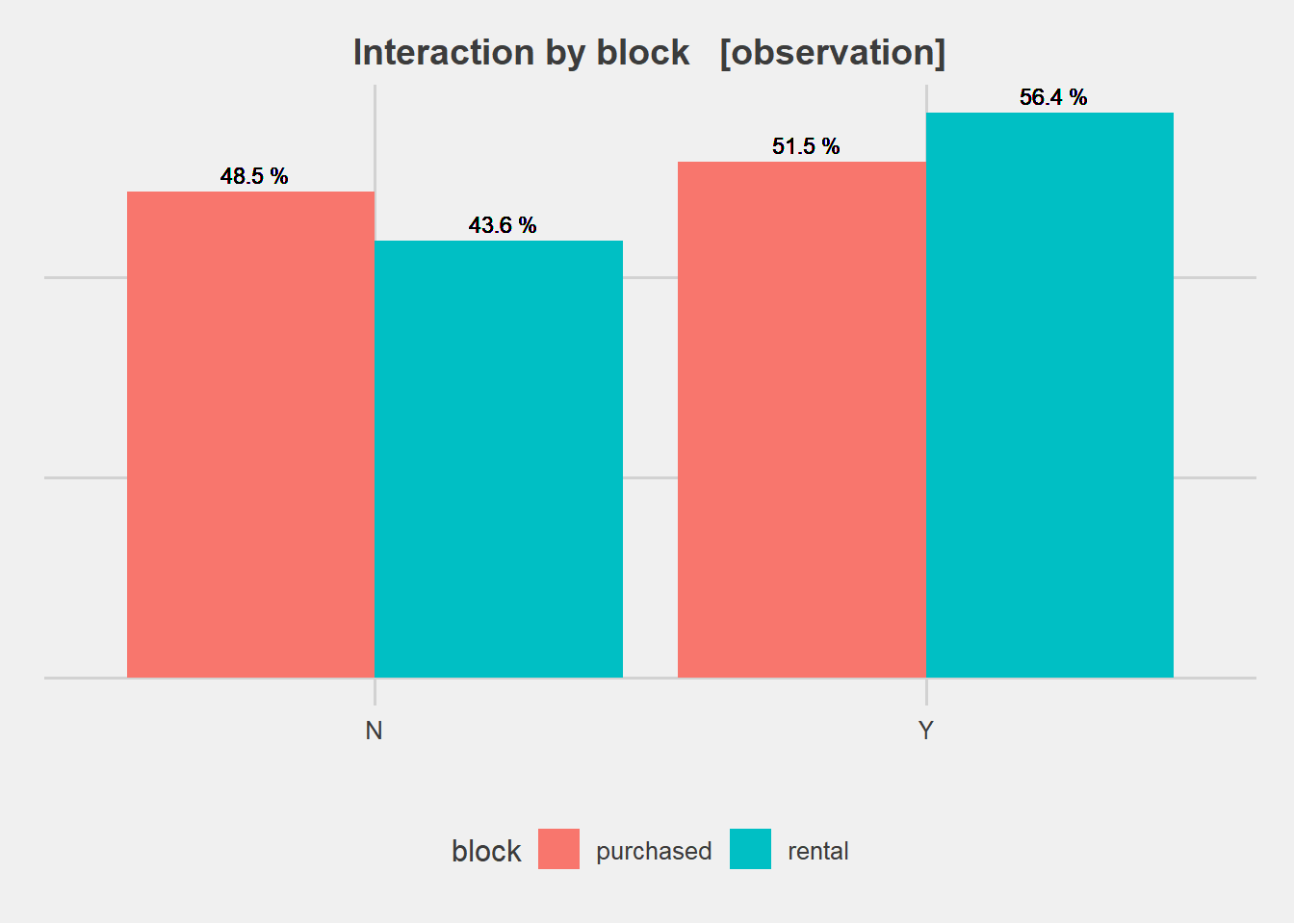
#ggsave("plots/interaction.png")1.8 Interaction intensity by block
observations %>%
  group_by(block) %>%
  mutate(total_block = n()) %>%
  group_by(interaction_intensity,block) %>%
  mutate(perc_label = paste(round(n()/total_block*100,1),"%")) %>%
  mutate(perc = n()/total_block*100) %>%
  ggplot(aes((interaction_intensity), fill=block))+
  geom_bar(aes(y = perc),stat="identity",position="dodge")+
  geom_text(aes(y=perc,label=perc_label),position=position_dodge(width=0.9),vjust=-0.5, hjust=0.43,size=3,color="black")+
  theme_fivethirtyeight() +
  labs(title="Interaction intensity by block   [observation]") +
  theme(plot.title = element_text(size=14, hjust=0.5))+
  theme(axis.title = element_text()) + xlab('') + ylab('percentage')+
  theme(axis.title.y=element_blank(),
        axis.text.y=element_blank(),
axis.ticks.y=element_blank()) 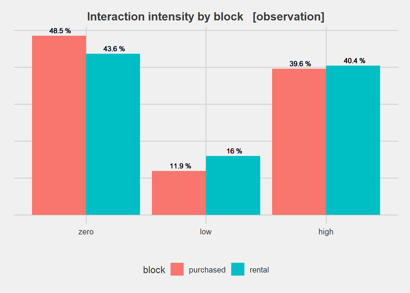
#ggsave("plots/intensity.png")1.9 Interaction intensity by time per block
observations %>%
  mutate(hour=hour(date_time_in)) %>%
  group_by(block) %>%
  mutate(total_block = n()) %>%
  group_by(hour, block, interaction_intensity) %>%
  mutate(perc_label = paste(round(n()/total_block*100,1),"%")) %>%
  mutate(perc = round(n()/total_block*100,1)) %>%
  ggplot(aes(as.factor(hour), interaction_intensity, alpha=perc)) + geom_tile() +
  theme_fivethirtyeight() +
  labs(title="Interaction intensity by hour of day per block   [observation]") +
  theme(plot.title = element_text(size=14, hjust=0.5))+
  theme(axis.title = element_text()) + xlab('hour') + ylab('interaction intentsity') +
  scale_x_discrete(breaks=c("9","10","11","12","13","14","15","16","17","18","19"),
        labels=c("09:00","10:00","11:00","12:00","13:00","14:00","15:00","16:00","17:00","18:00","19:00"))+
  facet_grid(block~.)+
  theme(panel.spacing = unit(3, "lines"))+
  theme(axis.text.x = element_text(angle = 90, hjust = 1, vjust = 0.5))+
  guides(alpha=FALSE)+
  aes(fill = block)+
  geom_text(aes(label=perc_label, alpha=1),size=2)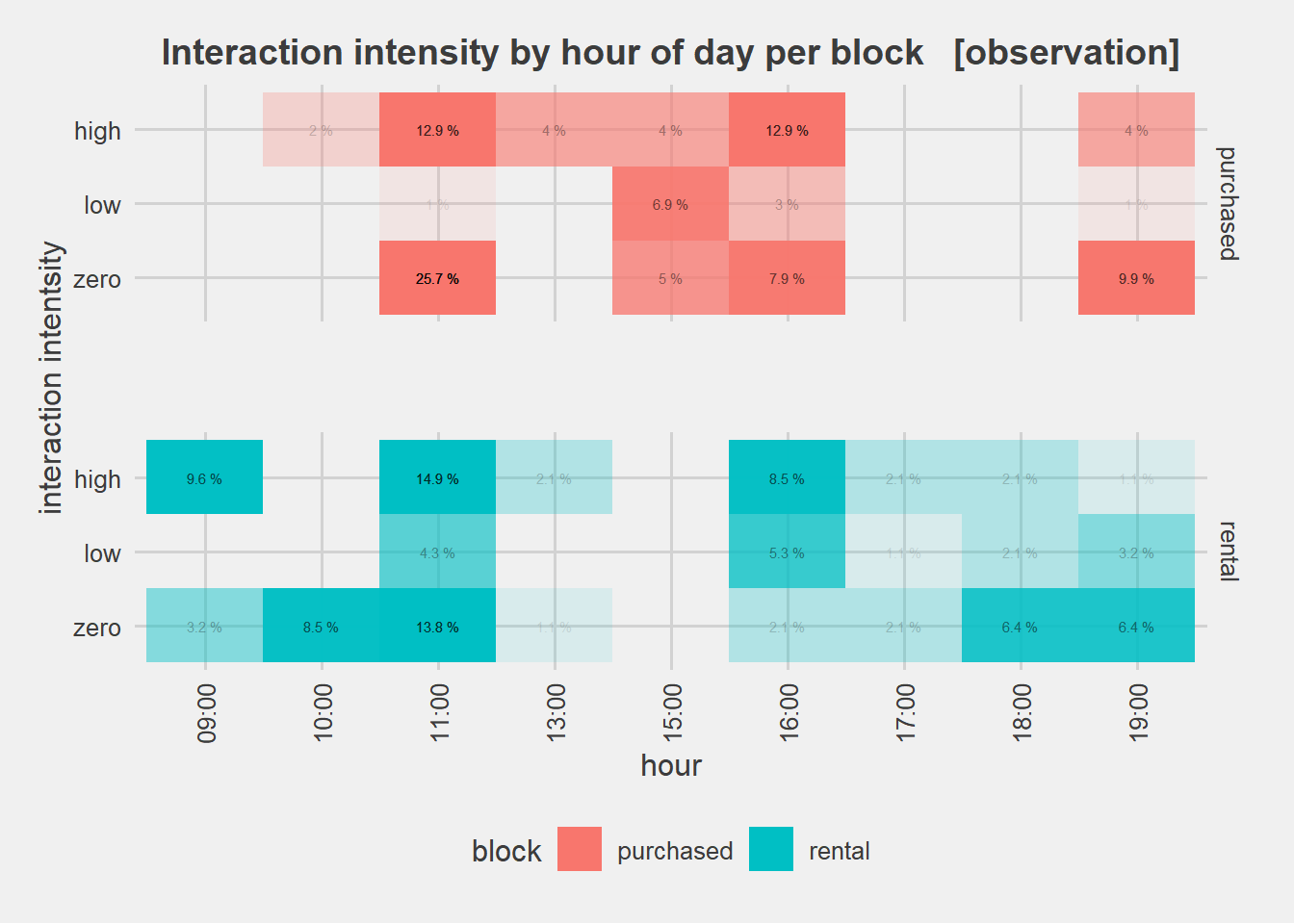
#ggsave("plots/hourly_intensity.png")1.10 Table of count and percentage of interaction intensity
table <- observations %>%
  filter(interaction_intensity!="zero") %>%
  filter(block=="rental") %>%
  group_by(block) %>%
  mutate(total_block = n()) %>%
  group_by(planned_or_spontaneous,duration_intensity,verbal_or_non_verbal,majority_in_same_grid,interaction_intensity) %>%
  mutate(count=n()) %>%
  mutate(`percentage (%)`=(round((count/total_block*100),2))) %>%
  select(c("block","planned_or_spontaneous","duration_intensity","verbal_or_non_verbal","majority_in_same_grid","interaction_intensity","count","percentage (%)")) %>%
  distinct() %>%
  rename("duration intensity"=duration_intensity,
         "majority in same grid"=majority_in_same_grid,
         "interaction intensity"=interaction_intensity,
         "verbal or non-verbal"=verbal_or_non_verbal,
         "planned or spontaneous" = planned_or_spontaneous)%>%
  arrange(desc(`percentage (%)`))

customRed = "#ff7f7f"
customBlue = "#00bfc4"
formattable(table,
            align =c("l","c","c","c","c","c", "c", "r"),
            list(block = formatter(
              "span", style = ~ style(color = "grey",font.weight = "bold")),
`percentage (%)` = color_bar(customBlue)))| block | planned or spontaneous | duration intensity | verbal or non-verbal | majority in same grid | interaction intensity | count | percentage (%) |
|---|---|---|---|---|---|---|---|
| rental | planned | low | verbal | Y | high | 20 | 37.74 |
| rental | spontaneous | low | verbal | Y | high | 12 | 22.64 |
| rental | planned | low | non-verbal | Y | low | 11 | 20.75 |
| rental | spontaneous | low | non-verbal | Y | low | 4 | 7.55 |
| rental | planned | high | verbal | Y | high | 4 | 7.55 |
| rental | spontaneous | high | non-verbal | Y | high | 2 | 3.77 |
table <- observations %>%
  filter(interaction_intensity!="zero") %>%
  filter(block=="purchased") %>%
  group_by(block) %>%
  mutate(total_block = n()) %>%
  group_by(planned_or_spontaneous,duration_intensity,verbal_or_non_verbal,majority_in_same_grid,interaction_intensity) %>%
  mutate(count=n()) %>%
  mutate(`percentage (%)`=(round((count/total_block*100),2))) %>%
  select(c("block","planned_or_spontaneous","duration_intensity","verbal_or_non_verbal","majority_in_same_grid","interaction_intensity","count","percentage (%)")) %>%
  distinct() %>%
  rename("duration intensity"=duration_intensity,
         "majority in same grid"=majority_in_same_grid,
         "interaction intensity"=interaction_intensity,
         "verbal or non-verbal"=verbal_or_non_verbal,
         "planned or spontaneous" = planned_or_spontaneous) %>%
  arrange(desc(`percentage (%)`))


formattable(table,
            align =c("l","c","c","c","c","c", "c", "r"),
            list(block = formatter(
              "span", style = ~ style(color = "grey",font.weight = "bold")),
`percentage (%)` = color_bar(customRed)))| block | planned or spontaneous | duration intensity | verbal or non-verbal | majority in same grid | interaction intensity | count | percentage (%) |
|---|---|---|---|---|---|---|---|
| purchased | planned | low | verbal | Y | high | 28 | 53.85 |
| purchased | spontaneous | low | verbal | Y | high | 7 | 13.46 |
| purchased | spontaneous | low | non-verbal | Y | low | 4 | 7.69 |
| purchased | spontaneous | low | verbal | N | low | 4 | 7.69 |
| purchased | spontaneous | high | verbal | Y | high | 3 | 5.77 |
| purchased | planned | low | non-verbal | Y | low | 3 | 5.77 |
| purchased | planned | high | verbal | Y | high | 2 | 3.85 |
| purchased | spontaneous | high | non-verbal | N | low | 1 | 1.92 |
1.11 Age-group and interaction intensity for purchased block
table <- observations %>%
  filter(block=="purchased") %>%
  group_by(interaction_intensity,block) %>%
  mutate(total_interactionintensity_block = n()) %>%
  group_by(age_group,duration_intensity,interaction_intensity) %>%
  mutate(count=n()) %>%
  mutate(`percentage (%)`=(round((count/total_interactionintensity_block*100),2))) %>%
  select(c("age_group","duration_intensity","interaction_intensity","count","percentage (%)")) %>%
  distinct() %>%
  rename("duration intensity"=duration_intensity,
         "age group"=age_group,
         "interaction intensity"=interaction_intensity) %>%
  arrange(desc(`percentage (%)`)) %>%
  arrange(`interaction intensity`)


formattable(table,
            align =c("l","c","c","c","r"),
            list(block = formatter(
              "span", style = ~ style(color = "grey",font.weight = "bold")),
`percentage (%)` = color_bar(customRed)))| age group | duration intensity | interaction intensity | count | percentage (%) |
|---|---|---|---|---|
| 40 to 50 | low | zero | 17 | 34.69 |
| 30 to 40 | low | zero | 9 | 18.37 |
| 20 to 30 | low | zero | 8 | 16.33 |
| 50 to 65 | low | zero | 7 | 14.29 |
| 7 to 20 | low | zero | 2 | 4.08 |
| 20 to 30 | high | zero | 2 | 4.08 |
| below 7 | low | zero | 2 | 4.08 |
| 65 to 80 | low | zero | 1 | 2.04 |
| 50 to 65 | high | zero | 1 | 2.04 |
| 65 to 80 | low | low | 4 | 33.33 |
| below 7 | low | low | 2 | 16.67 |
| 20 to 30 | low | low | 2 | 16.67 |
| 30 to 40 | low | low | 2 | 16.67 |
| 40 to 50 | low | low | 1 | 8.33 |
| 40 to 50 | high | low | 1 | 8.33 |
| 30 to 40 | low | high | 9 | 22.50 |
| 50 to 65 | low | high | 9 | 22.50 |
| 40 to 50 | low | high | 5 | 12.50 |
| 20 to 30 | low | high | 4 | 10.00 |
| below 7 | low | high | 4 | 10.00 |
| 65 to 80 | low | high | 3 | 7.50 |
| 50 to 65 | high | high | 2 | 5.00 |
| 7 to 20 | low | high | 1 | 2.50 |
| 40 to 50 | high | high | 1 | 2.50 |
| 7 to 20 | high | high | 1 | 2.50 |
| below 7 | high | high | 1 | 2.50 |
table <- kableExtra::kable(table)%>%
  kable_styling(full_width = F) %>%
  group_rows("No interaction", 1, 9) %>%
  group_rows("Low interaction", 10, 15) %>%
  group_rows("High interaction", 16, 26)

table| age group | duration intensity | interaction intensity | count | percentage (%) |
|---|---|---|---|---|
| No interaction | ||||
| 40 to 50 | low | zero | 17 | 34.69 |
| 30 to 40 | low | zero | 9 | 18.37 |
| 20 to 30 | low | zero | 8 | 16.33 |
| 50 to 65 | low | zero | 7 | 14.29 |
| 7 to 20 | low | zero | 2 | 4.08 |
| 20 to 30 | high | zero | 2 | 4.08 |
| below 7 | low | zero | 2 | 4.08 |
| 65 to 80 | low | zero | 1 | 2.04 |
| 50 to 65 | high | zero | 1 | 2.04 |
| Low interaction | ||||
| 65 to 80 | low | low | 4 | 33.33 |
| below 7 | low | low | 2 | 16.67 |
| 20 to 30 | low | low | 2 | 16.67 |
| 30 to 40 | low | low | 2 | 16.67 |
| 40 to 50 | low | low | 1 | 8.33 |
| 40 to 50 | high | low | 1 | 8.33 |
| High interaction | ||||
| 30 to 40 | low | high | 9 | 22.50 |
| 50 to 65 | low | high | 9 | 22.50 |
| 40 to 50 | low | high | 5 | 12.50 |
| 20 to 30 | low | high | 4 | 10.00 |
| below 7 | low | high | 4 | 10.00 |
| 65 to 80 | low | high | 3 | 7.50 |
| 50 to 65 | high | high | 2 | 5.00 |
| 7 to 20 | low | high | 1 | 2.50 |
| 40 to 50 | high | high | 1 | 2.50 |
| 7 to 20 | high | high | 1 | 2.50 |
| below 7 | high | high | 1 | 2.50 |
1.12 Age-group and interaction intensity for rental block
table <- observations %>%
  filter(block=="rental") %>%
  group_by(interaction_intensity,block) %>%
  mutate(total_interactionintensity_block = n()) %>%
  group_by(age_group,duration_intensity,interaction_intensity) %>%
  mutate(count=n()) %>%
  mutate(`percentage (%)`=(round((count/total_interactionintensity_block*100),2))) %>%
  select(c("age_group","duration_intensity","interaction_intensity","count","percentage (%)")) %>%
  distinct() %>%
  rename("duration intensity"=duration_intensity,
         "age group"=age_group,
         "interaction intensity"=interaction_intensity) %>%
  arrange(desc(`percentage (%)`)) %>%
  arrange(`interaction intensity`)


table <- formattable(table,
            align =c("l","c","c","c","r"),
            list(block = formatter(
              "span", style = ~ style(color = "grey",font.weight = "bold")),
              `percentage (%)` = color_bar(customRed)))
table <- kable(table)%>%
  kable_styling(full_width = F) %>%
  group_rows("No interaction", 1, 8) %>%
  group_rows("Low interaction", 9, 14) %>%
  group_rows("High interaction", 15, 23)

table| age group | duration intensity | interaction intensity | count | percentage (%) |
|---|---|---|---|---|
| No interaction | ||||
| 20 to 30 | low | zero | 11 | 26.83 |
| 30 to 40 | low | zero | 9 | 21.95 |
| 40 to 50 | low | zero | 8 | 19.51 |
| 50 to 65 | low | zero | 5 | 12.20 |
| 65 to 80 | low | zero | 4 | 9.76 |
| 7 to 20 | low | zero | 2 | 4.88 |
| 20 to 30 | high | zero | 1 | 2.44 |
| below 7 | low | zero | 1 | 2.44 |
| Low interaction | ||||
| 20 to 30 | low | low | 5 | 33.33 |
| 50 to 65 | low | low | 2 | 13.33 |
| below 7 | low | low | 2 | 13.33 |
| 65 to 80 | low | low | 2 | 13.33 |
| 30 to 40 | low | low | 2 | 13.33 |
| 40 to 50 | low | low | 2 | 13.33 |
| High interaction | ||||
| 30 to 40 | low | high | 10 | 26.32 |
| 40 to 50 | low | high | 8 | 21.05 |
| 20 to 30 | low | high | 7 | 18.42 |
| 50 to 65 | low | high | 4 | 10.53 |
| 30 to 40 | high | high | 3 | 7.89 |
| below 7 | low | high | 2 | 5.26 |
| 50 to 65 | high | high | 2 | 5.26 |
| 7 to 20 | low | high | 1 | 2.63 |
| 65 to 80 | high | high | 1 | 2.63 |
1.13 Planned or spontaneous interaction by block
observations %>%
  filter(planned_or_spontaneous!="NA") %>%
  group_by(block) %>%
  mutate(total_block = n()) %>%
  group_by(planned_or_spontaneous,block) %>%
  mutate(perc_label = paste(round(n()/total_block*100,1),"%")) %>%
  mutate(perc = n()/total_block*100) %>%
  ggplot(aes((planned_or_spontaneous), fill=block))+
  geom_bar(aes(y = perc),stat="identity",position="dodge")+
  geom_text(aes(y=perc,label=perc_label),position=position_dodge(width=0.9),vjust=-0.5, hjust=0.43,size=3,color="black")+
  theme_fivethirtyeight() +
  labs(title="Nature of interactions by block   [observation]") +
  theme(plot.title = element_text(size=14, hjust=0.5))+
  theme(axis.title = element_text()) + xlab('') + ylab('percentage')+
  theme(axis.title.y=element_blank(),
        axis.text.y=element_blank(),
axis.ticks.y=element_blank()) 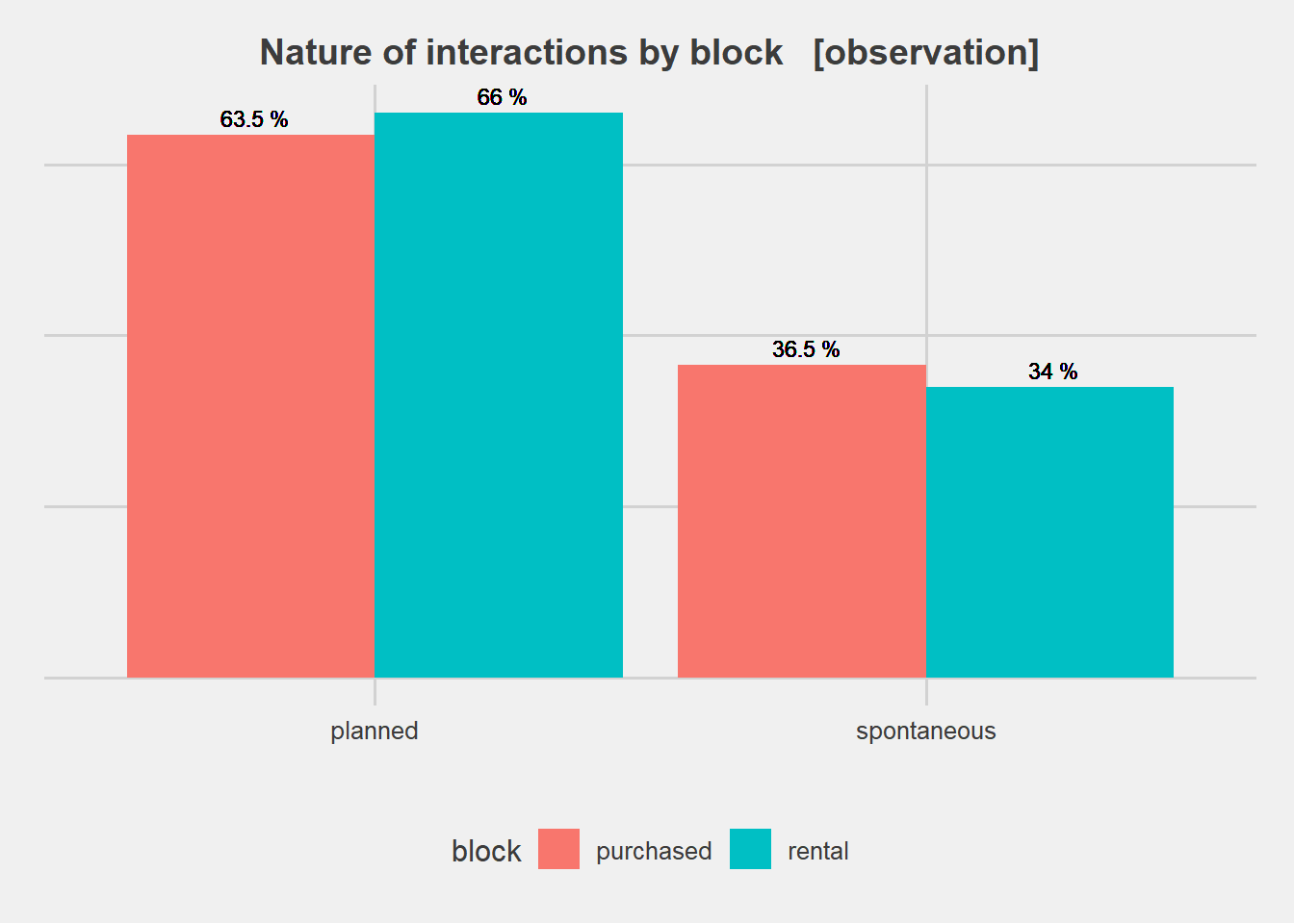
#ggsave("plots/planned_or_chance.png")