Chapter 7 Chi Squared
7.1 There are two ways to run a Chi Square test. This walk-through will go through both with a couple of examples.
Say we had two cohorts, “Control” and “Experimental”
set.seed(1)
Cohorts <- sample(c("Control", "Experimental"), size = 1000, replace = TRUE)
Each cohort will also have the binary variable of sex assigned to them, as well as a categorical variable of age ranges.
set.seed(2)
Sex <- sample(c("Male", "Female"), size = 1000, replace = TRUE)

set.seed(3)
Age.Range <- sample(c("20-29", "30-39", "40-49", "50-59"), size = 1000, replace = TRUE)

Data.Frame <- as.data.frame(cbind(Cohorts, Sex, Age.Range))
rm(Cohorts, Age.Range, Sex)
To test of our two cohorts differ significantly from one another with regards to sex or age range, we use the chi square test of independence. The first step is to create a contingency table from our data (ie a summary table with the number of males and females in each cohort). We will save the contingency table.
table(Data.Frame$Cohorts, Data.Frame$Sex)##
## Female Male
## Control 249 253
## Experimental 255 243Cont.Sex <- table(Data.Frame$Cohorts, Data.Frame$Sex)Now, we run the chi square test of independence. Note that continuity correction is typically applied when any of the numbers in the contingency table are below 10 (some say 5). Fisher’s Exact test may also be another option. However, this is a non-issue for our current sample.
chisq.test(Cont.Sex, correct = F)##
## Pearson's Chi-squared test
##
## data: Cont.Sex
## X-squared = 0.25705, df = 1, p-value = 0.6122We can do the same thing for the age ranges as we did for sex, even though age ranges has more than two options
Cont.Age <- table(Data.Frame$Cohorts, Data.Frame$Age.Range)
chisq.test(Cont.Age)
##
## Pearson's Chi-squared test
##
## data: Cont.Age
## X-squared = 2.2822, df = 3, p-value = 0.5159The alternative option to the above is to give the chisq.test function two vectors and it will calculate the contingency table behind the scenes. This is obviously less code, but is less straightforward to me and typically you will want to see the contingency table anyways.
chi.vectors <- chisq.test(Data.Frame$Cohorts, Data.Frame$Sex, correct = F)
chi.vectors$observed
## Data.Frame$Sex
## Data.Frame$Cohorts Female Male
## Control 249 253
## Experimental 255 243chi.vectors$expected## Data.Frame$Sex
## Data.Frame$Cohorts Female Male
## Control 253.008 248.992
## Experimental 250.992 247.008chi.vectors$p.value## [1] 0.6121572chi.df <- chisq.test(Cont.Sex, correct = F)
chi.df$observed##
## Female Male
## Control 249 253
## Experimental 255 243chi.df$expected##
## Female Male
## Control 253.008 248.992
## Experimental 250.992 247.008chi.df$p.value## [1] 0.6121572Finally, let’s say that you have the contingency table already in excel and just want to run the chi square test as quickly and easily as possible. You don’t want to manually enter the data into R, and you don’t want to deal with excels statistics functionality.
Easy! Copy the contingency table into your clipboard (just exclude the row names):
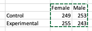
Then, run the following (I’ve commented it out because it throws an error, but trust me it works):
#Cont.From.Xl <- read.delim(pipe("pbpaste"))
#chisq.test(Cont.From.Xl, correct = F)