1 Machine Learning Week 1: Linear and Multiple Regression
In machine learning, we use statistical and algorithmic strategies to detect patterns in our data. There are, generally, three goals: the first is to describe or understand our data. What are the patterns? How can we make sense of them? The second is to model our data - that is to apply a theory to our data about how it was generated and to evaluate the accuracy of that theory. Related, to two, the third goal is to make predictions - if our model is generalizable, then it should apply to other, but similar, situations. There are a number of strategies for identifying and modeling patterns in data.
In this regard, machine learning differs from more traditional ways of instructing computers on how to do things in that it provides a framework for the machine to learn from data on its own. We don’t have to type in what the machine should do at every step - it will be able to identify patterns using a model of choice across many different domains.
We will focus this week on Linear Regression, the most common startegy for identifying (linear) patterns in data and for modeling data. It is commonly used in social scientific studies to explain pheneomenon.
1.1 Batter up
The movie Moneyball focuses on the “quest for the secret of success in baseball”. It follows a low-budget team, the Oakland Athletics, who believed that underused statistics, such as a player’s ability to get on base, betterpredict the ability to score runs than typical statistics like home runs, RBIs (runs batted in), and batting average. Obtaining players who excelled in these underused statistics turned out to be much more affordable for the team.
In this lab we’ll be looking at data from all 30 Major League Baseball teams and examining the linear relationship between runs scored in a season and a number of other player statistics. Our aim will be to summarize these relationships both graphically and numerically in order to find which variable, if any, helps us best predict a team’s runs scored in a season.
1.2 The data
Let’s load up the data for the 2011 season.
download.file("http://www.openintro.org/stat/data/mlb11.RData", destfile = "mlb11.RData")
load("mlb11.RData")
summary(mlb11)
## team runs at_bats hits
## Arizona Diamondbacks: 1 Min. :556.0 Min. :5417 Min. :1263
## Atlanta Braves : 1 1st Qu.:629.0 1st Qu.:5448 1st Qu.:1348
## Baltimore Orioles : 1 Median :705.5 Median :5516 Median :1394
## Boston Red Sox : 1 Mean :693.6 Mean :5524 Mean :1409
## Chicago Cubs : 1 3rd Qu.:734.0 3rd Qu.:5575 3rd Qu.:1441
## Chicago White Sox : 1 Max. :875.0 Max. :5710 Max. :1600
## (Other) :24
## homeruns bat_avg strikeouts stolen_bases
## Min. : 91.0 Min. :0.2330 Min. : 930 Min. : 49.00
## 1st Qu.:118.0 1st Qu.:0.2447 1st Qu.:1085 1st Qu.: 89.75
## Median :154.0 Median :0.2530 Median :1140 Median :107.00
## Mean :151.7 Mean :0.2549 Mean :1150 Mean :109.30
## 3rd Qu.:172.8 3rd Qu.:0.2602 3rd Qu.:1248 3rd Qu.:130.75
## Max. :222.0 Max. :0.2830 Max. :1323 Max. :170.00
##
## wins new_onbase new_slug new_obs
## Min. : 56.00 Min. :0.2920 Min. :0.3480 Min. :0.6400
## 1st Qu.: 72.00 1st Qu.:0.3110 1st Qu.:0.3770 1st Qu.:0.6920
## Median : 80.00 Median :0.3185 Median :0.3985 Median :0.7160
## Mean : 80.97 Mean :0.3205 Mean :0.3988 Mean :0.7191
## 3rd Qu.: 90.00 3rd Qu.:0.3282 3rd Qu.:0.4130 3rd Qu.:0.7382
## Max. :102.00 Max. :0.3490 Max. :0.4610 Max. :0.8100
## In addition to runs scored, there are seven traditionally used variables in the data set: at-bats, hits, home runs, batting average, strikeouts, stolen bases, and wins. There are also three newer variables: on-base percentage, slugging percentage, and on-base plus slugging. For the first portion of the analysis we’ll consider the seven traditional variables. At the end of the lab, you’ll work with the newer variables on your own.
What type of plot would you use to display the relationship between runs and one of the other numerical variables? Plot this relationship using the variable at_bats as the predictor. Does the relationship look linear? If you knew a team’s at_bats, would you be comfortable using a linear model to predict the number of runs?
A scatter plot is good starting point to visualize runs vs. at bats.
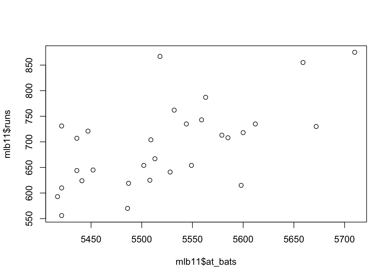
If the relationship looks linear, we can quantify the strength of the relationship with the correlation coefficient.
## [1] 0.6106271.3 Sum of squared residuals
Think back to the way that we described the distribution of a single variable. Recall that we discussed characteristics such as center, spread, and shape. It’s also useful to be able to describe the relationship of two numerical variables, such as runs and at_bats above.
Looking at your plot from the previous exercise, describe the relationship between these two variables. Make sure to discuss the form, direction, and strength of the relationship as well as any unusual observations. The relationships is linear; we can draw a straight line through the data with almost equal numbers of data points on the both side of the line. The relationship is strong there is scatter, but there is a definite slope to the trend line.
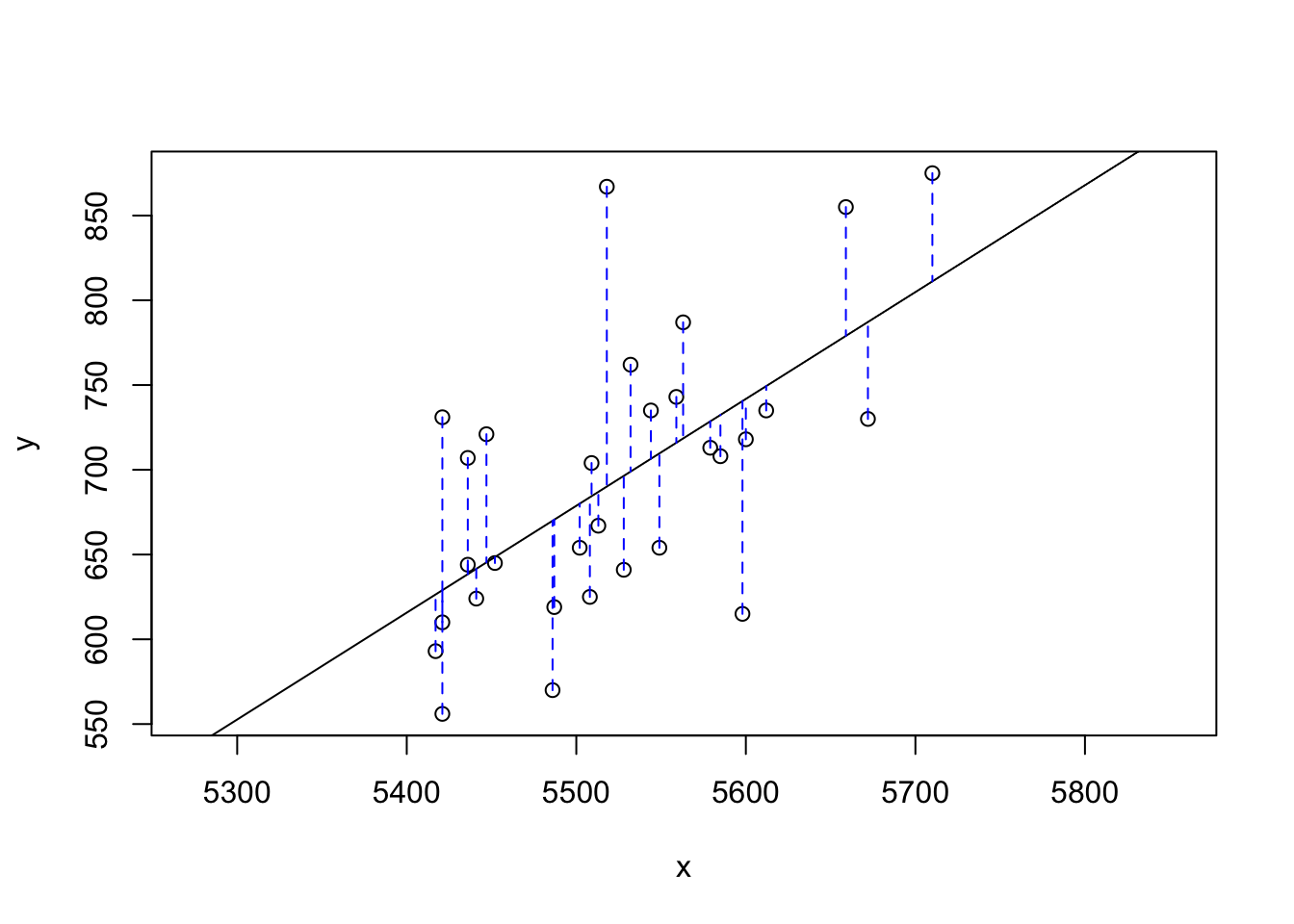
Just as we used the mean and standard deviation to summarize a single variable, we can summarize the relationship between these two variables by finding the line that best follows their association. Use the following interactive function to select the line that you think does the best job of going through the cloud of points.
## Click two points to make a line.

## Call:
## lm(formula = y ~ x, data = pts)
##
## Coefficients:
## (Intercept)            x
##  -2789.2429       0.6305
##
## Sum of Squares:  123721.9
After running this command, you’ll be prompted to click two points on the plot to define a line. Once you’ve done that, the line you specified will be shown in black and the residuals in blue. Note that there are 30 residuals, one for each of the 30 observations. Recall that the residuals are the difference between the observed values and the values predicted by the line:
- ei=yi−ŷi
## Click two points to make a line.
## Call:
## lm(formula = y ~ x, data = pts)
##
## Coefficients:
## (Intercept) x
## -2789.2429 0.6305
##
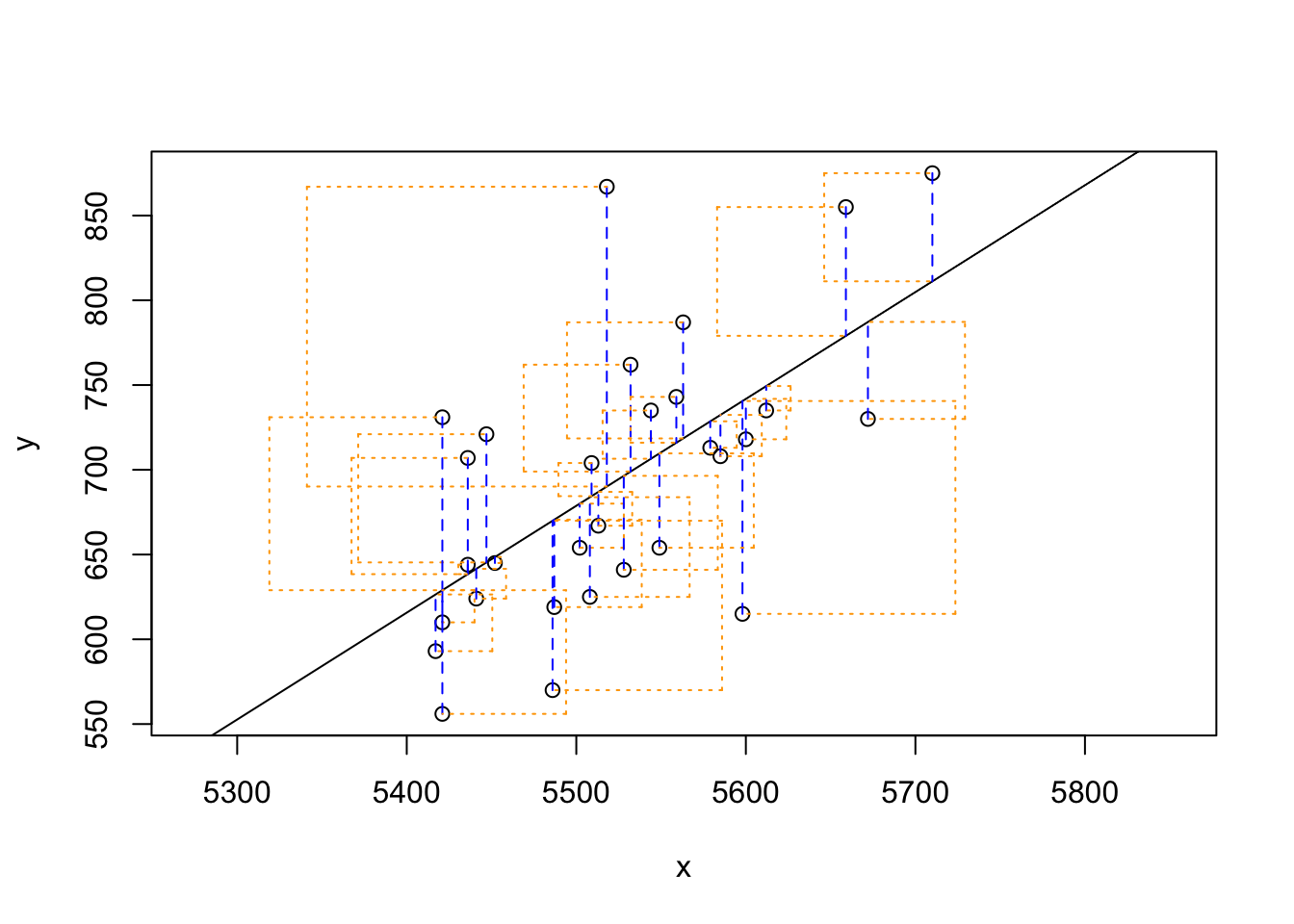
## Sum of Squares: 123721.9Note that the output from the plot_ss function provides you with the slope and intercept of your line as well as the sum of squares.
Using plot_ss, choose a line that does a good job of minimizing the sum of squares. Run the function several times. What was the smallest sum of squares that you got? How does it compare to your neighbors?

## Click two points to make a line.

## Call:
## lm(formula = y ~ x, data = pts)
##
## Coefficients:
## (Intercept)            x
##  -2789.2429       0.6305
##
## Sum of Squares:  123721.9
1.4 The linear model
It is rather cumbersome to try to get the correct least squares line, i.e. the line that minimizes the sum of squared residuals, through trial and error. Instead we can use the lm function in R to fit the linear model (a.k.a. regression line). It uses an algorithm, called gradient descent, to find the best fit line.
The first argument in the function lm is a formula that takes the form y ~ x. Here it can be read that we want to make a linear model of runs as a function of at_bats. The second argument specifies that R should look in the mlb11 data frame to find the runs and at_bats variables.
The output of lm is an object that contains all of the information we need about the linear model that was just fit. We can access this information using the summary function.
##
## Call:
## lm(formula = runs ~ at_bats, data = mlb11)
##
## Residuals:
## Min 1Q Median 3Q Max
## -125.58 -47.05 -16.59 54.40 176.87
##
## Coefficients:
## Estimate Std. Error t value Pr(>|t|)
## (Intercept) -2789.2429 853.6957 -3.267 0.002871 **
## at_bats 0.6305 0.1545 4.080 0.000339 ***
## ---
## Signif. codes: 0 '***' 0.001 '**' 0.01 '*' 0.05 '.' 0.1 ' ' 1
##
## Residual standard error: 66.47 on 28 degrees of freedom
## Multiple R-squared: 0.3729, Adjusted R-squared: 0.3505
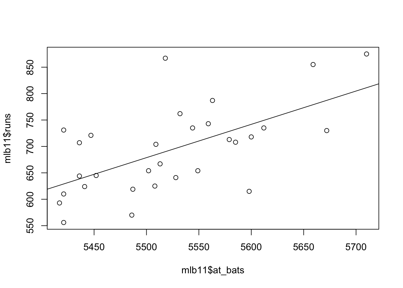
## F-statistic: 16.65 on 1 and 28 DF, p-value: 0.0003388Let’s consider this output piece by piece. First, the formula used to describe the model is shown at the top. After the formula you find the five-number summary of the residuals. The “Coefficients” table shown next is key; its first column displays the linear model’s y-intercept and the coefficient of at_bats. With this table, we can write down the least squares regression line for the linear model:
- ŷ=−2789.2429+0.6305∗atbats
One last piece of information we will discuss from the summary output is the Multiple R-squared, or more simply, R2. The R2 value represents the proportion of variability in the response variable that is explained by the explanatory variable. For this model, 37.3% of the variability in runs is explained by at-bats.
Fit a new model that uses homeruns to predict runs. Using the estimates from the R output, write the equation of the regression line. What does the slope tell us in the context of the relationship between success of a team and its home runs?
##
## Call:
## lm(formula = mlb11$runs ~ mlb11$homeruns)
##
## Residuals:
##     Min      1Q  Median      3Q     Max
## -91.615 -33.410   3.231  24.292 104.631
##
## Coefficients:
##                Estimate Std. Error t value Pr(>|t|)
## (Intercept)    415.2389    41.6779   9.963 1.04e-10 ***
## mlb11$homeruns   1.8345     0.2677   6.854 1.90e-07 ***
## ---
## Signif. codes:  0 '***' 0.001 '**' 0.01 '*' 0.05 '.' 0.1 ' ' 1
##
## Residual standard error: 51.29 on 28 degrees of freedom
## Multiple R-squared:  0.6266, Adjusted R-squared:  0.6132
## F-statistic: 46.98 on 1 and 28 DF,  p-value: 1.9e-07
y=415.2389+1.8345∗homeruns
The more home runs a team has the more successful the team
1.5 Prediction and prediction errors
Let’s create a scatterplot with the least squares line laid on top.
1.6 Model diagnostics
To assess whether the linear model is reliable, we need to check for (1) linearity, (2) nearly normal residuals, and (3) constant variability.
Linearity: You already checked if the relationship between runs and at-bats is linear using a scatterplot. We should also verify this condition with a plot of the residuals vs. at-bats. Recall that any code following a # is intended to be a comment that helps understand the code but is ignored by R.
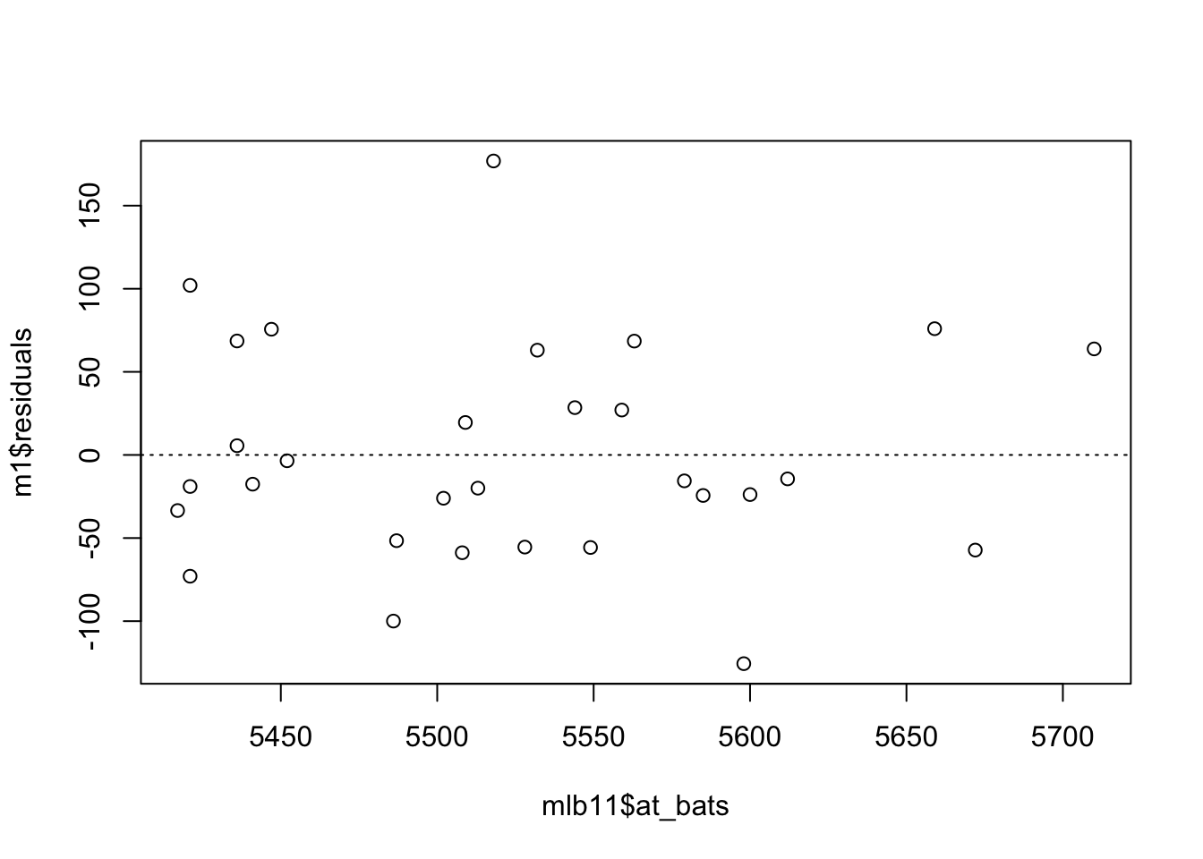
Is there any apparent pattern in the residuals plot? What does this indicate about the linearity of the relationship between runs and at-bats?
Answer: There is no pattern in the residuals. The data seems fairly evenly distributed above and below the trend line.
Nearly normal residuals: To check this condition, we can look at a histogram
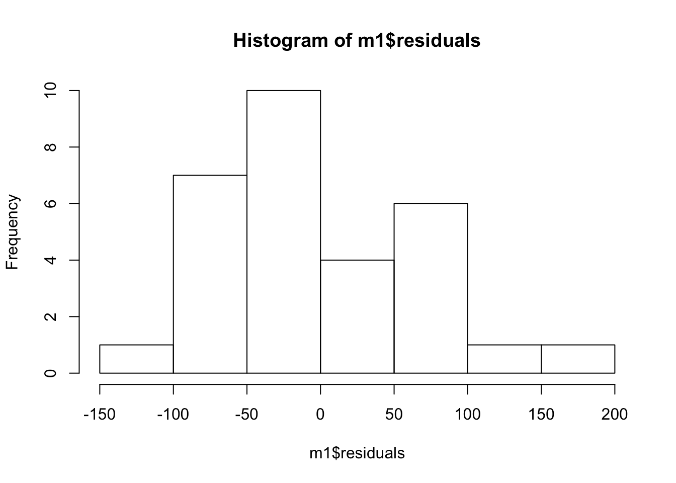
or a normal probability plot of the residuals.
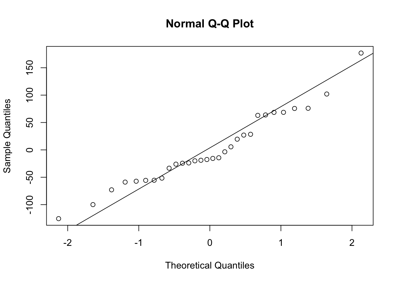
Based on the histogram and the normal probability plot, does the nearly normal residuals condition appear to be met? Answer: The models are valid and the QQ Normal plot seems to follow the theoretical values. Hence, the normal residual condition have been met.
Constant variability: Based on the plot in (1), does the constant variability condition appear to be met? Answer: When the residuals are plotted they randomly vary form -100 to 100 with the exception of 1 point at 150. variability condition seems like fulfilled
1.7 Multiple Regression
We can build more complex models by adding variables to our model. When we do that, we go from the world of simple regression to the more complex world of multiple regression.
Here, for example, is a traditional model with multiple different variables.
##
## Call:
## lm(formula = runs ~ homeruns + hits + strikeouts + bat_avg +
##     stolen_bases, data = mlb11)
##
## Residuals:
##     Min      1Q  Median      3Q     Max
## -33.615 -24.607   3.939  18.454  39.710
##
## Coefficients:
##                Estimate Std. Error t value Pr(>|t|)
## (Intercept)  -633.79390  234.50986  -2.703  0.01243 *
## homeruns        1.23355    0.16567   7.446  1.1e-07 ***
## hits           -0.05382    0.37949  -0.142  0.88840
## strikeouts      0.04222    0.06232   0.677  0.50457
## bat_avg      4357.92572 2648.84144   1.645  0.11296
## stolen_bases    0.51726    0.17232   3.002  0.00618 **
## ---
## Signif. codes:  0 '***' 0.001 '**' 0.01 '*' 0.05 '.' 0.1 ' ' 1
##
## Residual standard error: 27.42 on 24 degrees of freedom
## Multiple R-squared:  0.9085, Adjusted R-squared:  0.8895
## F-statistic: 47.67 on 5 and 24 DF,  p-value: 1.091e-11
What do we learn? How does the Multiple R-Squared look compard to previous models? Did we improve our model fit?
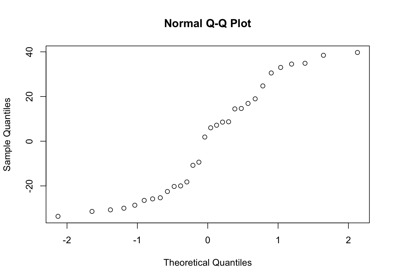
Let’s also verify that the conditions for this model are reasonable using diagnostic plots.
If our goal is to fit a more parsimonious model, we can drop the variable with the highest p-value and re-fit the model. Interestingly, in this case, the variable is hits. Did the coefficients and significance of the other explanatory variables change? (One of the things that makes multiple regression interesting is that coefficient estimates depend on the other variables that are included in the model.) If not, what does this say about whether or not the dropped variable was collinear with the other explanatory variables?
##
## Call:
## lm(formula = runs ~ homeruns + strikeouts + bat_avg + stolen_bases,
##     data = mlb11)
##
## Residuals:
##     Min      1Q  Median      3Q     Max
## -33.582 -24.759   3.683  18.081  39.891
##
## Coefficients:
##                Estimate Std. Error t value Pr(>|t|)
## (Intercept)  -615.46316  191.80651  -3.209  0.00364 **
## homeruns        1.23309    0.16236   7.595 5.98e-08 ***
## strikeouts      0.04153    0.06090   0.682  0.50155
## bat_avg      3991.64541  577.25566   6.915 3.01e-07 ***
## stolen_bases    0.51800    0.16883   3.068  0.00512 **
## ---
## Signif. codes:  0 '***' 0.001 '**' 0.01 '*' 0.05 '.' 0.1 ' ' 1
##
## Residual standard error: 26.88 on 25 degrees of freedom
## Multiple R-squared:  0.9084, Adjusted R-squared:  0.8938
## F-statistic: 62.02 on 4 and 25 DF,  p-value: 1.296e-12
Let’s do it one more time.
##
## Call:
## lm(formula = runs ~ homeruns + bat_avg + stolen_bases, data = mlb11)
##
## Residuals:
##     Min      1Q  Median      3Q     Max
## -36.852 -23.209   4.842  19.974  36.590
##
## Coefficients:
##               Estimate Std. Error t value Pr(>|t|)
## (Intercept)  -507.4109   106.9704  -4.743 6.62e-05 ***
## homeruns        1.2541     0.1578   7.950 1.99e-08 ***
## bat_avg      3741.2846   440.8539   8.486 5.75e-09 ***
## stolen_bases    0.5210     0.1670   3.119   0.0044 **
## ---
## Signif. codes:  0 '***' 0.001 '**' 0.01 '*' 0.05 '.' 0.1 ' ' 1
##
## Residual standard error: 26.6 on 26 degrees of freedom
## Multiple R-squared:  0.9067, Adjusted R-squared:  0.896
## F-statistic: 84.27 on 3 and 26 DF,  p-value: 1.613e-13
Now that we have a parsimonious model using traditional predictors, let’s add in some of the new variables that the Oakland A’s made use of. We can do this one at time to see how it affects the significance and magnitude of the other coefficients. This informs us of which variables the new variable is collinear with.
##
## Call:
## lm(formula = runs ~ homeruns + bat_avg + stolen_bases + new_onbase,
##     data = mlb11)
##
## Residuals:
##     Min      1Q  Median      3Q     Max
## -43.505 -12.550  -0.913  12.289  33.020
##
## Coefficients:
##               Estimate Std. Error t value Pr(>|t|)
## (Intercept)  -808.0220   101.8224  -7.936 2.72e-08 ***
## homeruns        0.9345     0.1353   6.908 3.06e-07 ***
## bat_avg      1147.7956   640.1101   1.793  0.08506 .
## stolen_bases    0.3879     0.1271   3.051  0.00534 **
## new_onbase   3197.9060   678.4307   4.714 7.83e-05 ***
## ---
## Signif. codes:  0 '***' 0.001 '**' 0.01 '*' 0.05 '.' 0.1 ' ' 1
##
## Residual standard error: 19.74 on 25 degrees of freedom
## Multiple R-squared:  0.9506, Adjusted R-squared:  0.9427
## F-statistic: 120.3 on 4 and 25 DF,  p-value: 6.008e-16
On-base percentage (new_onbase) appears to attenuate the significance of batting average. Let’s add slugging percentage.
m7 <- lm(runs ~ homeruns + bat_avg + stolen_bases + new_onbase + new_slug, data = mlb11)
summary(m7)
##
## Call:
## lm(formula = runs ~ homeruns + bat_avg + stolen_bases + new_onbase +
## new_slug, data = mlb11)
##
## Residuals:
## Min 1Q Median 3Q Max
## -44.06 -14.16 1.03 10.84 36.19
##
## Coefficients:
## Estimate Std. Error t value Pr(>|t|)
## (Intercept) -786.1971 102.0182 -7.706 6.08e-08 ***
## homeruns 0.4140 0.4296 0.964 0.344784
## bat_avg -44.8496 1129.0434 -0.040 0.968642
## stolen_bases 0.3274 0.1342 2.440 0.022459 *
## new_onbase 3004.9260 686.9796 4.374 0.000204 ***
## new_slug 1077.2624 844.9179 1.275 0.214518
## ---
## Signif. codes: 0 '***' 0.001 '**' 0.01 '*' 0.05 '.' 0.1 ' ' 1
##
## Residual standard error: 19.5 on 24 degrees of freedom
## Multiple R-squared: 0.9538, Adjusted R-squared: 0.9441
## F-statistic: 99 on 5 and 24 DF, p-value: 3.247e-15Interestingly, it isn’t significant itself but appears to reduce the significance of the a few of the other variables. Did the coefficients change much? R2 is approaching 0.95 - rarely will you find an R2 this high anywhere in the social world! Of course, baseball is just a game..
1.8 Prediction
Finally, imagine that a new baseball team joined the MLB. We collected some data on them over their first season and now want to predict how many runs they are likely to get in their next season.
Here is the new team. They are, by design, totally average across every variable, much like my Colorado Rockies. We will call them the San Jose Sluggers.
## Warning in mean.default(x, na.rm = T): argument is not numeric or logical:
## returning NAAs long as a data.frame has the same variables as those in a model, we can use the predict function to predict the expected outcomes of the respondents in the data.frame using the model. How many runs with this team get? How does it compare to the average number of runs teams got in 2011?
##     1
## 693.6## [1] 693.6