11 Communication

11.1 Information Theory

11.1.1 Entropy

Most of the examples are taken from philentropy package in R, which can be accessed via this link

11.1.1.1 Discrete Entropy

If $\mathbf{p}_X = (p_{x1},p_{x2},...,p_{xn})$ is the probability distribution of the discrete random variable X with $P(X = x) = p_{xi}$. Then, the entropy of the distribution is (Shannon 1948)

$$H(\mathbf{p}_X) = -\sum_{x_i} p_{xi}\log_2 p_{xi}$$

where

• entropy unit is bits, and $H(p) \in [0,1]$ and max at $p = 0.5$
• or the unit is nats ($log_e$)
• or the unit is dits ($log_{10}$)

In general, if you have different bases, you can convert between units. Given bases a and b

$$\log_a k = \log_a b \times log_b k$$

where $\log_a b$ is a constant.

Generalize

$$H_b(X) = log_b a \times H_a(X)$$

Equivalently,

$$H(X) = E(\frac{1}{\log p(x)})$$

Entropy is the measure of how much information gained from learning the value of X (Zwillinger 1995, 262). Entropy depends on the distribution of X.

Example:

If X has 2 values, then $\mathbf{p}= (p,1-p)$ and

$$H(\mathbf{p}_X ) = H(p,1-p) = -p \log_2 p - (1-p) \log_2 (1-p)$$

which is known as binary entropy function

Plot of p vs. H(p) where max of $H(\mathbf{p}_X) = \log_2 n$ when $X \sim U$

hb <- function(gamma) {
    -gamma * log2(gamma) - (1 - gamma) * log2(1 - gamma) # output in bits
}

xs <- seq(0, 1, len = 100)
plot(xs,
     hb(xs),
     type = 'l',
     xlab = "p",
     ylab = "H(p)")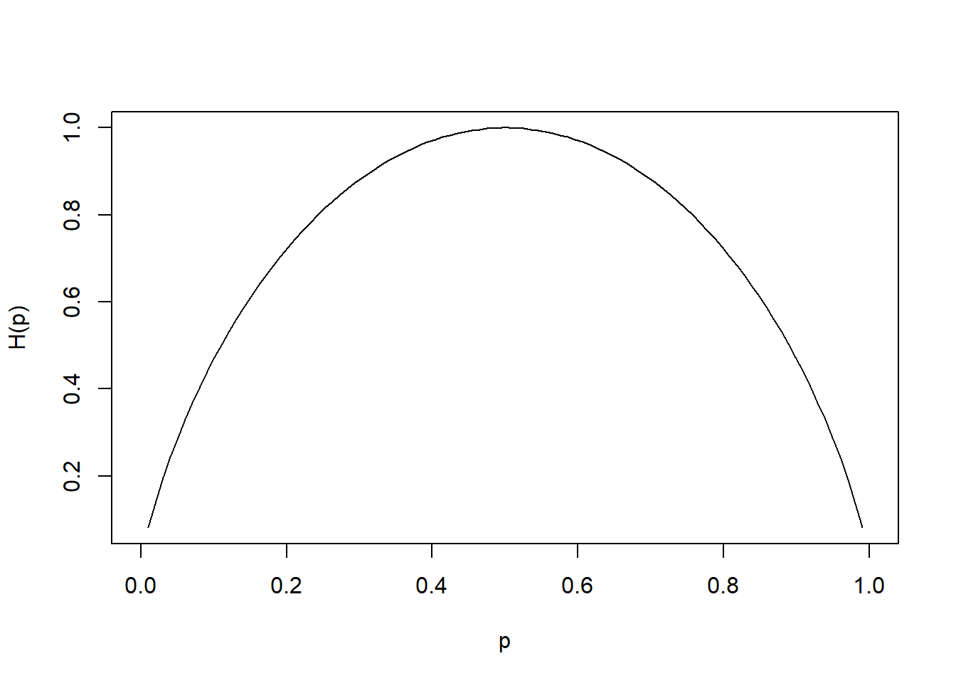

library("philentropy")
Prob <- 1:10/sum(1:10) # probabilities P(X)
H(Prob) # Shannon's Entropy

## [1] 3.103643

11.1.1.2 Mutual Information

If X and Y are two discrete random variables and $\mathbf{p}_{X \times Y}$ is the their joint distribution, the mutual information (i.e., learning of a value of X gives information about the value of Y) of X and Y is

$$I(X,Y) = I(Y,X) = H(\mathbf{p}_X)+ H(\mathbf{p}_Y)- H(\mathbf{p}_{X \times Y})$$

where $I(X,Y) \ge 0$ and $I(X,Y) = 0$ iff X and Y are independent (information about X gives no information about Y).

Equivalently,

$$MI(X,Y) = \sum_{i=1}^n \sum_{j=1}^m P(x_i, y_j) \times \log_b (\frac{P(x_i,y_j)}{P(x_i) \times P(y_j)})$$

Properties:

• $I(X;X) = H(X)$ known as self-information
• $I(X;Y) \ge 0$ with equality iff $X \perp Y$

P_x <- 1:10/sum(1:10) # distribution P(X)
P_y <- 20:29/sum(20:29) # distribution P(Y)
P_xy <- 1:10/sum(1:10) # joint distribution P(X,Y)
MI(P_x, P_y, P_xy) # Mutual Information

## [1] 3.311973

11.1.1.3 Relative Entropy

The measure of the distance between distribution p and q is called relative entropy, denoted by $D(p ||q)$

Equivalently, it measures the inefficiency of assuming distribution q when the true distribution is p.

The relative entropy between p(x) and q(x) is

$$D(p||q) = \sum_x p(x) \log \frac{p(x)}{q(X)}$$

where

• $D(p||q) \ge 0$ and equality iff $p = q$

11.1.1.4 Joint-Entropy

$$H(X,Y) = - \sum_{i=1}^n \sum_{j = 1}^m P(x_i, y_j) \times \log_b(P(x_i,y_j))$$

P_xy <- 1:10/sum(1:10) # joint distribution P(X,Y)
JE(P_xy) # Joint-Entropy

## [1] 3.103643

11.1.1.5 Conditional Entropy

$$H(Y|X) = - \sum_{i=1}^n \sum_{j = 1}^m P(x_i, y_j) \times \log_b(\frac{P(x_i)}{P(x_i,y_j)})$$

P_x <- 1:10/sum(1:10) # distribution P(X)
P_y <- 1:10/sum(1:10) # distribution P(Y)
CE(P_x, P_y) # Joint-Entropy

## [1] 0

Relation among entropy measures

$$H(X,Y) = H(X) + H(Y|X) = H(Y) + H(X|Y)$$

Properties:

• Chain rule: $H(X_1, ..., X_n) = \sum_{i=1}^n H(X_i | X_{i-1},...,X_1)$
• $0 \le H(Y|X) \le H(Y)$ Information on X does not increase the entropy measure of Y
• If $X \perp Y$, then $H(Y|X) = H(Y); H(X,Y) = H(X) + H(Y)$
• $H(X) \le log |n_X|$ where $n_X$ = number of elements in X
• $H(X) = \log (n_X)$ iff $X \sim U$
• $H(X_1,...,X_n) \le \sum_i^n H(X_i)$
• $H(X_1,...,X_n) = \sum_i^n H(X_i)$ iff $X_i$’s are mutually independent.

11.1.1.6 Continuous Entropy

If X is a continuous variable, its entropy is

$$h(\mathbf{X}) = - \int_{R^d} p(\mathbf{x})\log p(\mathbf{x}) dx$$

where d is the dimension of X.

If X and Y are continuous random variables with density functions $p(\mathbf{x})$ and $q(\mathbf{y})$, the relative entropy is

$$H(X,Y) = \int_{R^d} p(x) \log \frac{p(x)}{q(x)} dx$$

More advance analysis can be access here

11.1.2 Divergence

Three metrics for divergence can be found here:

• Kullback-Leibler
• Jensen-Shannon
• Generalized Jensen-Shannon

11.1.3 Channel Capacity

The information channel capacity of a discrete memoryless channel is

$$C = \max_{p(x)} I(X;Y)$$

which is the highest rate use at which information can be sent without much error.
More information can be found here