Chapter 3 Maximum Likelihood
So, remember that with maximum likelihood, we want to determine a distribution that best fits our data.
test
I assume you already have an intuituve understanding of what maximum likelihood is doing, and now I want to show you how you can programmatically do MLE. In a similar structure to the video, we will first jsut look at how we can calculate maximum likelihood for a simple normal distirbution, then apply it to regression models
3.0.1 MLE for random data
So, we will first just generate some random data from a specified distribution, and then see if we can reverse engineer the distribution using maximum likelihood.
Let’s generate 10 data point that are drawn from a distribution with mean (\(\mu\)) of \(0\) and varaince (\(\sigma\)) 1
## [1] -1.5312481 0.7163078 0.3149509 0.3991166 -0.7848094 -0.7860068
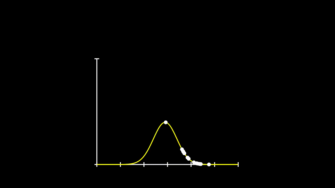
## [7] -0.6427575 0.1737502 -0.1698537 2.4400214Remember that calculating likelihood, just involved calculating the propobability of observing each given \(x\) value under a given distribution. So, lets fit some distributions to these data and see what their likelihood is.
y.all = seq(-3,3,0.1) #generating a list of values to build a curve
Pr = dnorm(y.all, mean = 0, sd = 0.5) #first curve has mean = 0 and sd = 0.2
Pr2 = dnorm(y.all, mean = 0.5, sd = 1) #second curve has mean = 0.5 and sd = 1
Pr3 = dnorm(y.all, mean = 0, sd = 1) #third curve has mean = 0.5 and sd = 1
plot(Pr ~ y.all, type = "l", ylim = c(0,0.8))
lines(Pr2 ~ y.all, type = "l", col = 36)
lines(Pr3 ~ y.all, type = "l", col = 21)
Pr.data = dnorm(data$y, mean = 0, sd = 0.5)
Pr.data2 = dnorm(data$y, mean = 0.5, sd = 1)
Pr.data3 = dnorm(data$y, mean = 0, sd = 1)
points(Pr.data~data$y)
points(Pr.data2~data$y)
points(Pr.data3~data$y)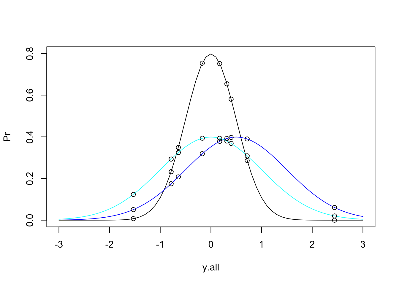
This gets a bit messy, but we can see that these data could come from any of these three distributions. So, if we want to determine the total likelihood of each of these distributions, we just need to calculate the product of the probabilities of each datum under the given distribution. The equation for our Total Likelihood for each distribution is:
\[ L(\mu, \sigma|x_1,\dots, x_n) = \prod_{i=1}^n\frac{1}{\sqrt{2\pi\sigma^2}}e^\frac{(x_i - \mu)^2}{2\sigma} \]
Fortunately, this normal distribution equation has a shortcut in R with the family of norm functions.
So, we will calulate the Likelihood of our data under three different distributions:
\[ y \sim \mathcal{N}(0,0.5) \\ y \sim \mathcal{N}(0.5,1) \\ y \sim \mathcal{N}(0,1) \]
Remember, we are calculating the product of each value (I am multiplying by a constant to account for very small values)
d1 = prod(dnorm(data$y, mean = 0, sd = 0.5)) * 10**6
d2 = prod(dnorm(data$y, mean = 0.5, sd = 1)) * 10**6
d3 = prod(dnorm(data$y, mean = 0, sd = 1)) * 10**6
cbind(d1,d2,d3)
## d1 d2 d3
## [1,] 4.566211e-05 0.1426874 0.4668093We see our data are more likely under the third distribution, which remember is the distribution we samples from originally. So, we expect that!
But is this distirbution, the MOST likeliy distribution for these data? Maybe, maybe not. We would need to sample every single combination of \(\mu\) and \(\sigma\) to be sure.
Similar to how we built an optimization function for least squares, we can do the same for MLE.
So, we first need to ask, which function do we want to optimize? You might say we want to optimize the liklihood function, and you would be right! Kinda…remember, that the likelihood function gets pretty tough to integrate, so we use the log liklihood. So, we will be optimizing the log-likelihood for data, with our unknown parameters being \(\mu\) and \(\sigma\).
loglik <- function(par,y){
  sum(dnorm(y, mean = par[1], sd = par[2], log = TRUE))
  #we are using sum because its the log, which converts multiplication to addition
}
Now we have specified a function to calculate the logplikelihood, so now we just need to tell R to optimize that function for us.
MLE <- optim(c(mu = 0, sigma = 1), fn = loglik, #parameters to be estimated, function to optimise
               y = data$y, control = list(fnscale = -1, reltol = 1e-16)
               #we specify -1 in the controls so that we MAXIMIZE rather than minimize, which is the default
               )
MLE$par
## mu sigma
## 0.01294713 1.03799052So, we find that the most likely distribution for our data is a population with mean \(0.0129\) and variance \(1.037\). Remember, the actual population we drew from had a mean of 0 and variance of 1, so this is certainly a reasonable estimate for a sample size of 10.
Now, we can compare what we got to what R’s built in ML Estimator glm() finds.
## [1] 0.01294714Our estimate for the mean is the same as the glm estimate. Let’s look at the estimate for the variance.
## [1] 1.037991You may be tempted to ask why I have multiplied the sigma by \(\sqrt\frac{n-1}{1}\). The answer is that MLE gives a biased estimate of sigma while OLS gives an unbiased estimate of sigma. Silly questions get silly answers. In other words this is a topic for a different video
For those interested, the difference in how variance is calculated in MLE vs OLS is the motivation for using Restricted Maximum Likliehood (REML)
3.1 MLE Regression
Okay, so we have a method for calculating ML estimates in R, so now we want to apply that to some regression models. Let’s return to our formula for linear model. Let’s use the same data fom our least squares example to see if we can get similar results.
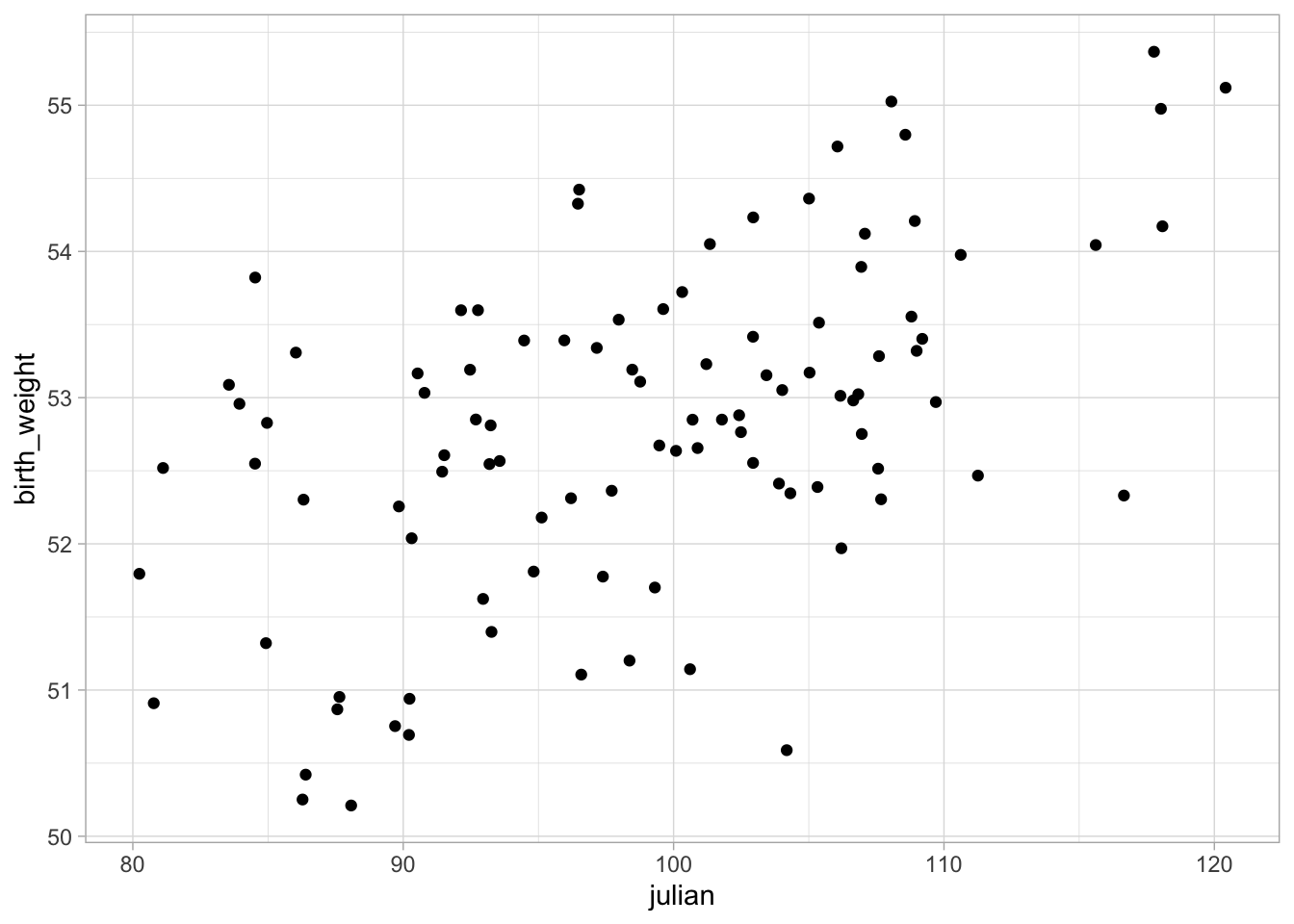
Let’s return to our linear model. We will start by looking at only a single predictor, mpg so our system of linear equations looks like this:
\[ E[y_i] = \beta_0 + \beta_1x_i \]
Recall from the video, we are assuming each datum is drawn from some distribution with a mean equal to \(\beta_0 + \beta_1x_1\).
So, this distribution, then becomes our distribution we are maximizing, where
\[ y_i \sim \mathcal{N}(\beta_0 + \beta_1x_i, \sigma) \]
Let’s try plugging this distribution into our loglik function to calculate the likelihood of this distribution.
loglikMLE <- function(par, y){
  x = as.vector(birth_data$julian)
  sum(dnorm(y, mean = par[1] + par[2]*x, sd = par[3], log = T))
}
MLE <- optim(c(intercept = 43, julian = 0, sigma = 1), fn = loglikMLE, #parameters to be estimated, function to optimise
y = as.vector(birth_data$birth_weight), control = list(fnscale = -1, reltol = 1e-16)
#we specify -1 in the controls so that we MAXIMIZE rather than minimize, which is the default
)
round(MLE$par,4)## intercept julian sigma
## 46.2863 0.0659 0.9544Fantastic! We have found similar parameter estimates to our least squares method! Lets see how this compares to what glm gives us.
## (Intercept)      julian
## 46.28632464 0.06588573## [1] 0.9640796n = length(birth_data$birth_weight)
X = dim(model.matrix(birth_data$birth_weight ~ birth_data$julian))[2]
sigma(glm(birth_weight ~ julian, data = birth_data)) * sqrt((n-X)/n)## [1] 0.9543901So what about applying this to multiple parameters? Well, let’s see. We will use the same model formula as our multiple parameter OLS:
birth_weight ~ julain + nest_temp
Which can be represented by the system of linear equations:
\[ E[y_i] = \beta\textbf{X} \]
This means each y value is drawn from some hypothetical distribution where:
\[ y_i \sim \mathcal{N}(\beta\textbf{X}, \sigma) \]
loglikmMLE <- function(par, y){
  x1 = as.vector(birth_data$julian)
  x2 = as.vector(birth_data$nest_temp)
  sum(dnorm(y, mean = par[1] + par[2]*x1 + par[3]*x2, sd = par[4], log = TRUE))
}set.seed(185)
MLE <- optim(c(intercept = 43, julian = 0, nest_temp = 0, sigma = 1), fn = loglikmMLE, #parameters to be estimated, function to optimise
y = as.vector(birth_data$birth_weight), control = list(fnscale = -1, reltol = 1e-16), hessian = TRUE
#we specify -1 in the controls so that we MAXIMIZE rather than minimize, which is the default
)
round(MLE$par,4)## intercept julian nest_temp sigma
## 48.0903 0.0665 -0.0627 0.9270And we can compare these results to glm.
n = length(birth_data$birth_weight)
X = dim(model.matrix(birth_data$birth_weight ~ birth_data$julian + birth_data$nest_temp))[2]
summary(glm(birth_weight ~ julian + nest_temp, data = birth_data, family = "gaussian"))$coefficients[,1]
## (Intercept) julian nest_temp
## 48.09032072 0.06649805 -0.06274910## [1] 0.92704073.1.1 Another tangent on optimizers
So one thing you may notice is that I specified the values where the algorithm should start looking for our parameter estimates
This is a result of us having at least a decent idea of where the idea minimum should be. What happens when we specify really bad starting values for the optimization algorithm?
set.seed(185)
MLE <- optim(c(intercept = 0, julian = 0, nest_temp = 0, sigma = 1), fn = loglikmMLE, #parameters to be estimated, function to optimise
               y = as.vector(birth_data$birth_weight), control = list(fnscale = -1, reltol = 1e-16), hessian = TRUE
               #we specify -1 in the controls so that we MAXIMIZE rather than minimize, which is the default
               )
round(MLE$par,4)
## intercept julian nest_temp sigma
## 40.3617 0.1031 0.0490 1.2426You see we find new optima. NOw what if we use a different optimization function
set.seed(185)
MLE <- optim(c(intercept = 0, julian = 0, nest_temp = 0, sigma = 1), fn = loglikmMLE, #parameters to be estimated, function to optimise
               y = as.vector(birth_data$birth_weight), control = list(fnscale = -1, reltol = 1e-16), method = "BFGS"
               #we specify -1 in the controls so that we MAXIMIZE rather than minimize, which is the default
               )
round(MLE$par,4)
## intercept julian nest_temp sigma
## 48.0903 0.0665 -0.0627 0.9270This optimizer does actually find the global maxima despite the bad starting values.
I firmly believe understanding optimizers will make anyone better at diagnosing the functionality of their linear models.