Example 3

Data: trees1.csv

This data set has been looked at in the lectures. The main question of interest is how to model the relationship between log(volume) (y) and log(diameter) (x1) and log(height) (x2), using data from 31 cherry trees.

To model the relationship we decided to go with the multiple linear regression model

\(Y_i = \alpha + \beta x_{1i} +\gamma x_{2i} + \epsilon_i\); \(\epsilon_i \approx N(0, \sigma^2);\) \(i = 1,..., 31\)

Set the working directory in RStudio to the directory in which you have stored both the data and R script by going to:

Session > Set Working Directory > To Source File Location

and read in the data using:

trees1 <- read.csv("trees1.csv")

Exploratory analysis

A matrix plot with scatter plots between each pair of variables can be used to gain an initial impression. This can be produced by using the following command in R:

pairs(trees1, lower.panel = NULL)

The argument lower.panel = NULL only displays the top diagonal of the matrix which ensures the response of log(volume) is on the y-axis of the plots. It may be more appropriate to use upper.panel = NULL depending on the position of the response variable in the dataframe. Figure 1 shows the relationships between the three variables.

trees1 <- read.csv("trees1.csv")
pairs(trees1, lower.panel = NULL)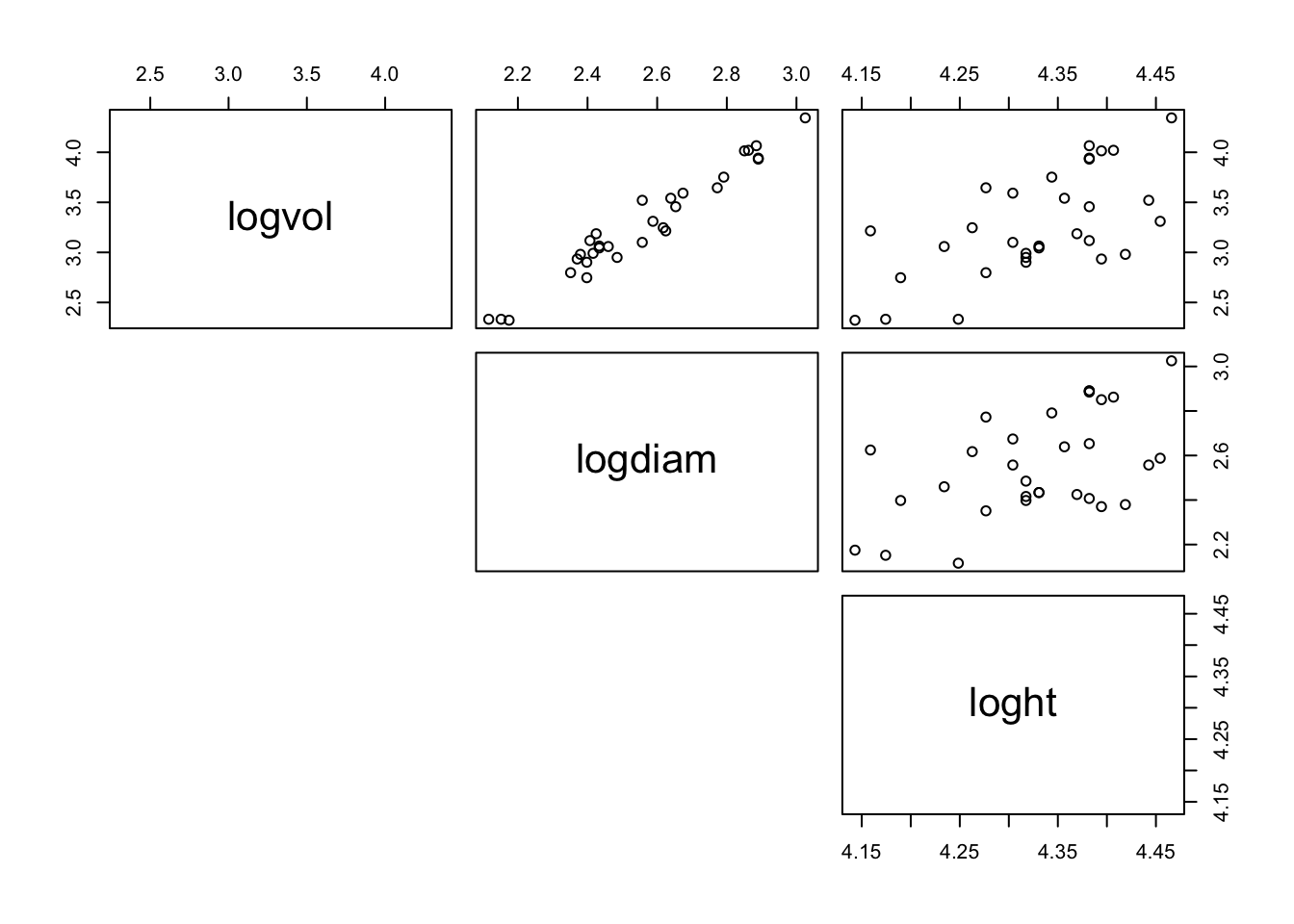

Figure 1: Scatter plot displaying the relationships between the three variables

Looking at figure 1 complete the sentences to best describe these scatter plots.

The Log volume against log diameter scatter plot shows a , association. There are no outliers in the data.

The Log volume against log height scatter plot shows a , association. There are no outliers in the data.

The Log diameter against log height scatter plot shows a , association. There are no outliers in the data.

Statistical analysis
We now fit the multiple linear regression model stated below

\(Y_i = \alpha + \beta x_{1i} +\gamma x_{2i} + \epsilon_i\); \(\epsilon_i \approx N(0, \sigma^2);\) \(i = 1,..., 31\)

in R using the following command:

Model1 <- lm(logvol ˜ logdiam + loght, data = trees1)

and produce residual plots to graphically assess the assumptions of the linear model using:

plot(rstandard(Model1) ˜ fitted(Model1)) qqnorm(rstandard(Model1))

par(mfrow = c(1, 2))
Model1 <- lm(logvol ~ logdiam + loght, data = trees1)
plot(rstandard(Model1) ~ fitted(Model1))
abline(h=0, lty=3)
qqnorm(rstandard(Model1))
abline(a=0, b=1, lty=3)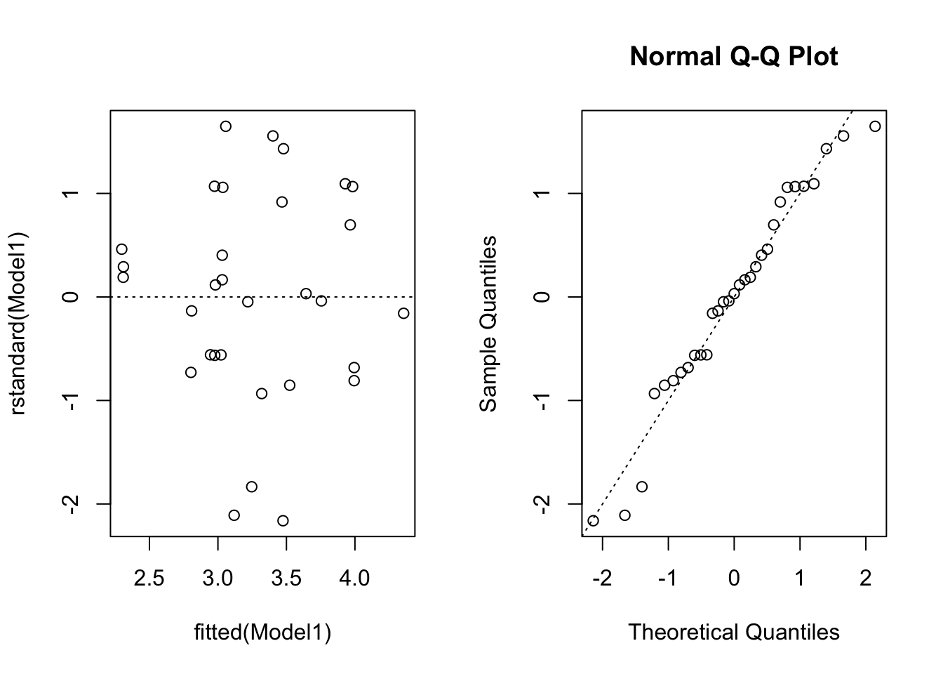

Figure 2: Residuals vs fitted values(left) and normal QQ-plot right

Figure 2 displays the residual plots after fitting a simple linear regression model to the transformed variables.The points are fairly evenly scattered above and below the zero line, which suggests it is reasonable to assume that the random errors have mean zero. The vertical variation of the points seems to be small for small fitted values. However, there are also less points in this case. It would be preferable if more data are available. In the normal probability plot, we see that points do not exactly lie on diagonal line. This indicates that the Normality assumption may not necessarily be satisfied.

Regression output

We can now examine the regression output by typing:

summary(Model1)

## 
## Call:
## lm(formula = logvol ~ logdiam + loght, data = trees1)
## 
## Residuals:
##       Min        1Q    Median        3Q       Max 
## -0.168561 -0.048488  0.002431  0.063637  0.129223 
## 
## Coefficients:
##             Estimate Std. Error t value Pr(>|t|)    
## (Intercept) -6.63162    0.79979  -8.292 5.06e-09 ***
## logdiam      1.98265    0.07501  26.432  < 2e-16 ***
## loght        1.11712    0.20444   5.464 7.81e-06 ***
## ---
## Signif. codes:  0 '***' 0.001 '**' 0.01 '*' 0.05 '.' 0.1 ' ' 1
## 
## Residual standard error: 0.08139 on 28 degrees of freedom
## Multiple R-squared:  0.9777, Adjusted R-squared:  0.9761 
## F-statistic: 613.2 on 2 and 28 DF,  p-value: < 2.2e-16

The above output highlights that 97.61% (R2 (adj)) of the variation in the log volume of the cherry trees is accounted for by the linear model with log diameter and log height as predictors – which is very good indeed. The analysis of variance (ANOVA) table can also be obtained using:

anova(Model1)

## Analysis of Variance Table
## 
## Response: logvol
##           Df Sum Sq Mean Sq F value    Pr(>F)    
## logdiam    1 7.9254  7.9254 1196.53 < 2.2e-16 ***
## loght      1 0.1978  0.1978   29.86 7.805e-06 ***
## Residuals 28 0.1855  0.0066                      
## ---
## Signif. codes:  0 '***' 0.001 '**' 0.01 '*' 0.05 '.' 0.1 ' ' 1

Hypothesis testing

The hypotheses being tested for each of the parameters here are:

\(H_0\) : \(\beta\) = 0/ \(\gamma\) = 0 vs. \(H_1\) : \(\beta\) \(\neq\) 0 / \(\gamma\) \(\neq\) 0

Since the p-values for logdiam and loght are both < 0:001 (indicated by the significance codes in R ‘***’), and hence < 0:05, the null hypothesis H_0 is rejected and we conclude that log(diameter) is a statistically significant predictor of log(volume) in addition to log(height), and log(height) is a statistically significant predictor of log(volume) in addition to log(diameter).

Confidence interval for \(b^{T} \hat \beta\)

From lectures, the formula for a 95% confidence interval for a linear combination of the model parameters is:

\(b^{T} \hat \beta \pm t(n-p;0.975) \cdot e.s.e(b^{T} \hat \beta)\)

or, more explicitly,

\(b^{T} \hat \beta \pm t(n-p;0.975) \sqrt{\frac{RSS}{N-P}b^T(X'X)^{-1}b}\)

A 95% confidence interval for \(\beta\), the coefficient of log(diameter), can be formed by taking the vector b to be

\[b= \left[ \begin{array}{ccc} 0\\ 1\\ 0\\ \end{array} \right]\]

From the regression output, we know that

RSS = 0.1855 n − p = 31 − 3 = 28

with βˆ (the coefficients, estimates of the model parameters) and the estimated standard errors for the parameters provided in the R output. It remains to find the 0.975th quantile of the t-distribution with 28 degrees of freedom, and we do this in R as follows:

qt(p = 0.975, df = 28)

which gives us

## [1] 2.048407

Calculations Therefore, a 95% confidence interval for can be found by computing: 1.98265 + 2.048407 * 0.07501 1.98265 - 2.048407 * 0.07501

Hence a 95% confidence interval for the coefficient of log(diameter) is (1.83, 2.14). As this interval does not contain 0, we conclude that the predictor log(diameter) makes a statistically significant contribution in addition to the predictor log(height) in explaining the variability in log(volume). Therefore log(diameter) is retained in the model, in addition to log(height). The coefficient for log(diameter) is highly likely to lie between 1.83 and 2.14.

These intervals can be computed for all estimated parameters simultaneously in R using the following command:

confint(Model1)

##                 2.5 %    97.5 %
## (Intercept) -8.269912 -4.993322
## logdiam      1.828998  2.136302
## loght        0.698353  1.535894

Confidence interval for the population mean response and prediction interval for a future response Once we have fitted the model of interest it may also be useful to compute further confidence and prediction intervals from the fitted model. For example,

a 95% confidence interval for the population mean response; and
a 95% prediction interval for the response of an individual member of the population.

Questions

Question 1). Suppose that we consider a population of cherry trees for which the log(diameter) is 2.4 and the log(height) is 4.3. Provide a 95% confidence interval for the mean log(volume) in this population of cherry trees. Interpret the interval.

Question 2) Suppose, now, that we wish to obtain a 95% prediction interval for an individual cherry tree in the population which has a log(diameter) of 2.4 and a log(height) of 4.3. Interpret the interval.

We use R to compute the required intervals.

Solutions

Question 1 – 95% confidence interval for the population mean:

predframe <- data.frame(logdiam = 2.4, loght = 4.3) predict(Model1, int = "c", newdata = predframe)

##        fit      lwr      upr
## 1 2.930373 2.894059 2.966686

The data.frame command creates a table; each column represents one variable and each row contains one set of values from each column. The predict command can produce both a confidence interval and a prediction interval. To obtain a confidence interval we use the argument int = "c".

Therefore we conclude that in a population of cherry trees for which the log(diameter) is 2.4 and the log(height) is 4.3 it is highly likely that the log(volume) would lie, on average, somewhere between 2.89 and 2.97.

Question 2 – 95% prediction interval for a future tree:

predict(Model1, int = "p", newdata = predframe)

##        fit      lwr      upr
## 1 2.930373 2.759752 3.100994

The argument int = "p" in the predict command provides a prediction interval based on the specified values in the new dataframe predframe. Therefore if a cherry tree with a log(diameter) of 2.4 and a log(height) of 4.3 were selected randomly from the population of cherry trees, it is highly likely that it would have a log volume of somewhere between 2.76 and 3.10. Comparing with the 95% confidence interval, the 95% prediction interval has a wider range.