Chapter 1 Getting Started
1.1 Goals of Segmentation
The medial temporal lobes (MTL) are comprised of several regions of interest (ROI) for perception and memory research, including the rhinal cortex, hippocampus, and parahippocampal cortex. To understand the relationship between grey matter volume in these MTL regions and specific cognitive processes, we need to determine these regions’ boundaries. This is achieved through the manual segmentation, or tracing, of MTL regions. Here, we will introduce segmentation based on the Olsen-Amaral-Palombo (OAP) protocol.
1.2 Required Tools for Segmentation
- What software is used in this segmentation guide?
ITK-Snap (download link here) is used as the primary segmentation software in this protocol manual. See section 1.3 Getting Started with ITK-Snap Software to learn more.
What tools do I need to follow this segmentation guide? We recommend using a drawing pad, tablet or a stylus pen for segmentation. A mouse can also be used, however. We recommend the link here.
Which anatomical plane is used for segmentation? Segmentation is done on the coronal view, which allows for the best visualization of the ROIs. The axial and horizontal views will also come in handy when differentiating between sulci in the brain.
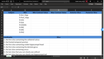
What other tools will I need for segmentation? You will also need a spreadsheet file for segmentation notes. This will include all your ROIs for each subject along with helpful notes about landmarks in the brain. Download our template here.
What type of scan do I use to segment under this protocol? The OAP protocol segments on T2-weighted images. T1 scans are used for anatomical reference.
1.3 First Steps in ITK-Snap
This section will help you get started with ITK-Snap for segmentation. Please note, you will need to first download the program (see the download link in 1.2 Required Tools for Segmentation).
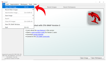
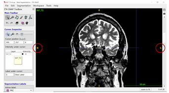
Step 1: Opening the T2 Image Open ITK-Snap by clicking on the program icon on your desktop or from the start menu. When the ITK-Snap window opens, select “File” from the top ribbon, then “Open Main Image” to open the T2-weighted image for a given subject.
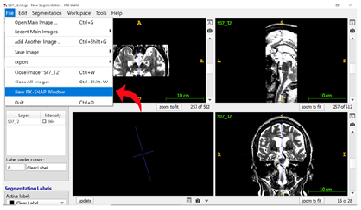
Step 2: Opening the T1 Image Select “File” from the top ribbon again, then click “New ITK-Snap Window” to open the T1-weighted image for the same subject.
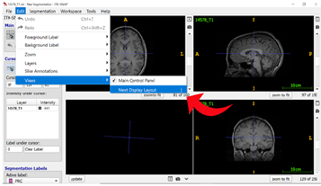
Step 3: Switching Between Views Since segmentation is done primarily on the coronal view of the T2-weighted image, you can easily switch between views using the shortcut SHIFT + | or by clicking “Edit” in the top ribbon and then “Views” in the dropdown menu to select “Next Display Layout” (see 6.1 ITK-Snap Shortcuts for more information).
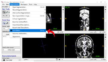
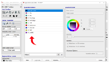
Step 4: Opening Label Editor On the T2-weighted image window, select “Segmentation” on the top ribbon and click on “Label Editor” to change your segmentation labels.
Step 5: Editing Labels Add the appropriate labels for MTL regions by typing each region’s name in the “Description” field, then selecting the colour for that region. You can learn more about naming conventions and the standard segmentation colours in the OAP protocol by reading section 1.5 Labels, Naming Conventions, and Contrasts.
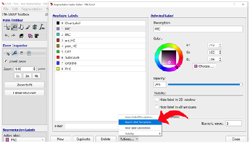
Step 6: Exporting Labels To make segmentation easier each time you re-open ITK-Snap, you can export and save your custom labels, which you can then import. See section 6.2 Label Import and Export for more information.
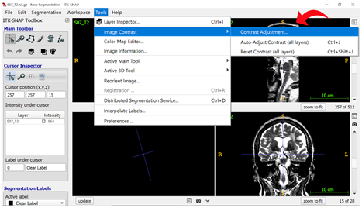
Step 7: Changing Image Contrasts To optimize the differentiation of gray matter from white matter, we can change the contrast on the T2 image. Select “Tools” in the top ribbon and click “Image Contrast”, then “Contrast Adjustment”.
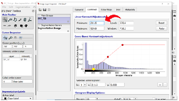
Step 8: Setting Image Contrasts As mentioned in step 7, you may need to adjust your image contrast to better see certain boundaries. We recommend a minimum contrast at approximately 200 and a maximum contrast at approximately 800 to 900. Be sure to record your contrast selection for each brain in your segmentation notes (see section 1.4 Lay of the Land for more information).
1.4 Lay of the Land
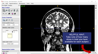
This section will help you get oriented and find the necessary landmarks to start segmenting. Step 1 will get you oriented with the T2 scan, while step 2 will help you find the landmarks for segmenting.
Part 1: Orientation
Before any segmentation is started, you must take note of the following:
- Screen Orientation: The left side of the screen is the right side of the brain (and vice versa).
- Slice Numbers: When you scroll through the slices, the slice number at the bottom right corner increases as you from anterior to posterior in the brain (and you will segment from anterior to posterior).
- Recording Landmarks: For both landmarks and ROIs, you will need to record relevant slice information and notes in the Segmentation Notes file (see section 1.2 Required Tools for Segmentation to download the file).
Part 2: Finding Landmarks
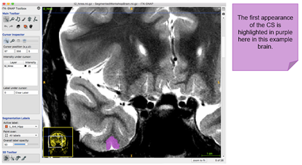
With your Segmentation Notes file open in a separate window, start by identifying the landmarks outlined in this section. It is critical that you follow the order outlined in this section, as certain earlier decisions on landmarks will inform later ones. Screenshots with examples are included to help you. Please note, however, that you will need to read the rules for each landmark carefully as your T2 files will certainly vary greatly!1. First slice containing the collateral sulcus
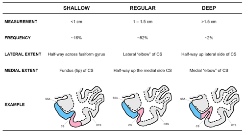
The first slice of the MTL is the first slice in your image set where you can clearly see the collateral sulcus. The grey matter ribbon only consists of the parahippocampal cortex. The depth of the collateral sulcus (CS) determines the medial and lateral borders of the perirhinal cortex. It is important to identify this first! Take a look at the example below:
The following table will help you determine the depth of the collateral sulcus in the brain you are segmenting. Examples are adapted from Insausti et al. (1998; see Section 8 Further Readings)
Careful, you might also run into cases where there is a double (or bifurcated) collateral sulcus. An estimated 25% to 35% of subjects will have a double collateral sulcus (Insausti et al., 1998; Pruessner et al., 2002). Note that not all slices in one subject may be a double collateral sulcus. In the examples below, B and C demonstrate interrupted and branched collateral sulci. These examples are adopted from Insausti et al. (1998):

What do you do about a double collateral sulcus when segmenting? The medial border should use the depth rules and the lateral border will extend until the fundus of the more lateral sulcus.
2. The Frontal-Temporal Junction
This key landmark will determine where you start drawing the entorhinal cortex. To find this landmark, look for the limen insulae. This is a band of grey matter that joins the frontal lobe to the temporal lobe. It is often easier to visualize on a T1-weighted scan. The two examples below compare a slice in which limen insulae is not visible, versus one that it is clearly visible: 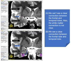
3. The first slice containing visible hippocampal head
Next, you will need to look for the hippocampal head. To find this landmark, keep these points in mind:
- In its first appearance, the hippocampal head will probably look like a “bean” shape
- The amygdala is located superior and the ventricle is lateral to the hippocampal head
- Ambient gyrus also appears in the same slice as the appearance of the hippocampal head
- Only draw one ROI for 2-3 slices until morphology of the hippocampus includes a visible C-shape on the lateral edge, at which point you can start segmenting subfields
In this section, we will be:
Surveying the goals of medial temporal lobe segmentation
Introducing ITK-Snap software for manual segmentation
Examining key regions of interest in the medial temporal lobes