A much more complete overview about loading and saving datasets of different formats is explained in How to load and save vector data in R, a weblog article in r-spatial. I will follow the tutorial in this article and comment it in difference to the GDSWR book.
A.1 Getting data
First of all I have to download the data to follow the tutorial.
R Code A.1 : Download data for the r-spatial tutorial
Code
## run this code chunk only once (manually)baseURL=here::here()pb_create_folder(base::paste0(baseURL, "/data/annex-a"))## download data into annex-a folderurl="https://github.com/kadyb/sf_load_save/archive/refs/heads/main.zip"utils::download.file(url, base::paste0(baseURL, "/data/annex-a/sf_load_save.zip"))utils::unzip(base::paste0(baseURL, "/data/annex-a/sf_load_save.zip"), exdir =base::paste0(baseURL, "/data/annex-a"))
(For this R code chunk is no output available)
A.2 Loading Shapefile (.shp)
It consists of several files (e.g., .shp, .shx, .dbf, .prj) that must be present in the same folder. Wikipedia has more details about this format. But this file format has many limitations and shouldn’t be used anymore.
Instead of using the base::getwd() and base::setwd() commands I am using here::here(), because it will always locate the files relative to the project root.
R Code A.2 : Load Shapefile
Code
## get path of r-spatial datar_spatial_path=base::paste0(here::here(), "/data/annex-a/sf_load_save-main/data/")## load and display the shapefile(countries=sf::read_sf(paste0(r_spatial_path, "countries/countries.shp")))
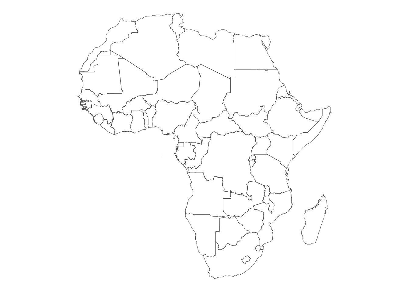
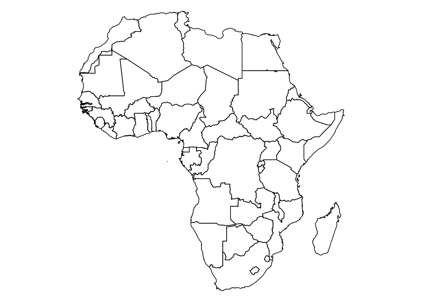
The countries object has many (168) fields (attributes), but to start with we only need the geometry column. Instead of using base::plot(countries$geometry) we can obtain geometry by using the sf::st_geometry() function.
A.3 Loading GeoPackage (.gpkg)
The next dataset is rivers (linear geometry) saved in GeoPackage format. It is loaded in exactly the same way as the shapefile before.
However, this format can consist of multiple layers of different types. In this case, we must define which layer exactly we want to load. To check what layers are in the geopackage, use the sf::st_layers() function, and then specify it using the layer argument in sf::read_sf(). If the file only contains one layer, we don’t need to do this.
R Code A.5 : Check layers of GeoPackage file
Code
## get path of r-spatial datar_spatial_path=base::paste0(here::here(), "/data/annex-a/sf_load_save-main/data/")sf::st_layers(base::paste0(r_spatial_path, "rivers.gpkg"))
#> Driver: GPKG
#> Available layers:
#>   layer_name     geometry_type features fields crs_name
#> 1     rivers Multi Line String      228     38   WGS 84
We can now load the rivers layers and display the metadata like in the shapefile example.
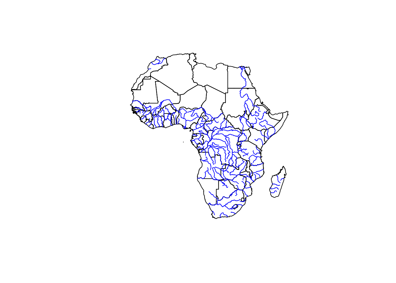
Visualizing the rivers data we we will plot this time the rivers against the background of country borders. Adding more layers to the visualization is done with the add = TRUE argument in the base::plot() function. Note that the order in which objects are added is important – the objects added last are displayed at the top. The col argument is used to set the color of the object.
Code Collection A.2 : Plotting rivers inside country borders
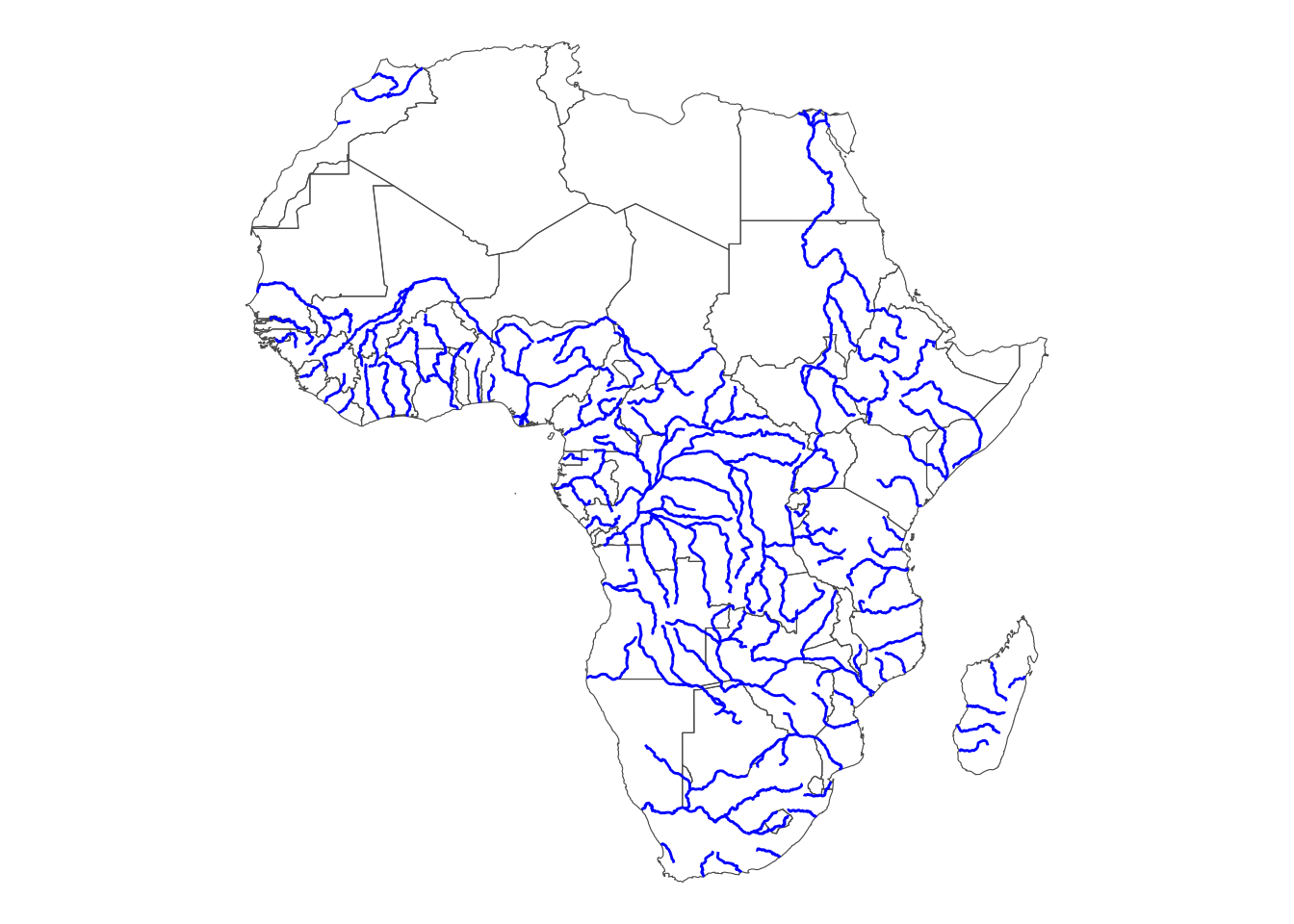
R Code A.8 : Visualizing rivers inside country borders using ggplot2::geom_sf()
Code
ggplot2::ggplot(data =countries)+ggplot2::geom_sf(fill =NA)+ggplot2::geom_sf(data =rivers, color ="blue")+ggplot2::theme_void()
Plotting rivers inside countriy borders with {ggplot2}
Adding more layers to the visualization is done in {ggplot2} as always with the + sign.
Note that the map is different (better) sized than the base::plot() example.
A.4 Loading GeoJSON (.geojson)
R Code A.9 : Loading GeoJSON cities file
Code
## get path of r-spatial datar_spatial_path=base::paste0(here::here(), "/data/annex-a/sf_load_save-main/data/")## load and display the GeoJSON file(cities=sf::read_sf(paste0(r_spatial_path, "cities.geojson")))
#> Simple feature collection with 1287 features and 1 field
#> Geometry type: POINT
#> Dimension:     XY
#> Bounding box:  xmin: -17.47508 ymin: -34.52953 xmax: 51.12333 ymax: 37.29042
#> Geodetic CRS:  WGS 84
#> # A tibble: 1,287 × 2
#>    featurecla                  geometry
#>    <chr>                    <POINT [°]>
#>  1 Admin-1 capital    (0.7890036 9.261)
#>  2 Admin-1 capital (0.9849965 8.557002)
#>  3 Admin-1 capital       (10.4167 33.4)
#>  4 Admin-1 capital     (8.971003 33.69)
#>  5 Admin-1 capital         (10.4667 33)
#>  6 Admin-1 capital      (10.2 36.86667)
#>  7 Admin-1 capital      (8.749999 36.5)
#>  8 Admin-1 capital   (8.716698 35.2167)
#>  9 Admin-1 capital   (9.500004 35.0167)
#> 10 Admin-1 capital   (9.383302 36.0833)
#> # ℹ 1,277 more rows
R Code A.11 : Print cities as text
Code
glue::glue("######## Using double square brackets #############")utils::head(cities[["featurecla"]])glue::glue("")glue::glue("############### Using dollar sign ##################")utils::head(cities$featurecla)
Tab “cities object” shows us that this layer contains 1287 different cities. To find out what types of cities these are, we can use the base::table() function, which will summarize them.
We are interested in Admin-0 capital and Admin-0 capital alt types because some countries have two capitals. I filtered the data using the | (OR) operator.
I am using the tidyverse approach with the native pipe instead of using base R as in the blog article.
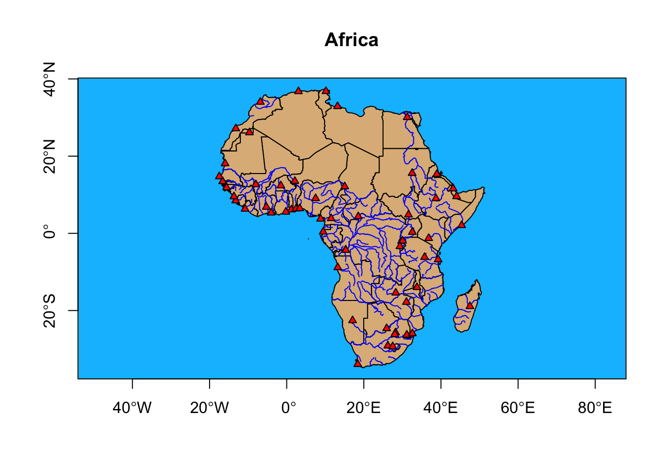
Code Collection A.4 : Plot Africa with rivers and capitals
In the last step, we prepare the final visualization.
R Code A.14 : Visualize African borders with rivers and capitals using base::plot()
Code
base::plot(sf::st_geometry(countries), main ="Africa", axes =TRUE, bgc ="deepskyblue", col ="burlywood")base::plot(sf::st_geometry(rivers), add =TRUE, col ="blue")base::plot(sf::st_geometry(capitals), add =TRUE, pch =24, bg ="red", cex =0.8)
We can add a title (main argument), axes (axes argument) and change the background color (bgc argument) of the figure. We can also change the point symbol (pch argument), set its size (cex argument) and fill color (bg argument).
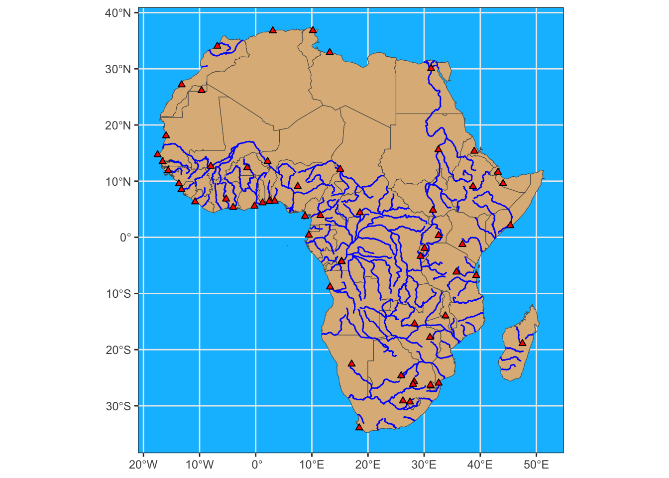
R Code A.15 : Visualize African borders with rivers and capitals
Code
ggplot2::ggplot(data =countries)+ggplot2::geom_sf(fill ="burlywood")+ggplot2::geom_sf(data =rivers, color ="blue")+ggplot2::geom_sf(data =capitals, fill ="red", shape =24)+ggplot2::theme( panel.background =ggplot2::element_rect(fill ="deepskyblue", color ="deepskyblue"))
Africa
This is essential the same map, but this time generated with {gplot2}.
Source Code
---knitr: opts_chunk: code-fold: show results: hold---# Load and save vector data in R {#sec-annex-a}```{r}#| label: setup#| results: hold#| include: falsebase::source(file ="R/helper.R")ggplot2::theme_set(ggplot2::theme_bw())```## Table of content for chapter 04 {.unnumbered}::::: {#obj-annex-a}:::: {.my-objectives}::: {.my-objectives-header}Chapter section list:::::: {.my-objectives-container}::::::::::::A much more complete overview about loading and saving datasets of different formats is explained in [How to load and save vector data in R](https://r-spatial.org/r/2024/06/26/sf-load-save.html), a weblog article in [r-spatial](https://r-spatial.org/). I will follow the tutorial in this article and comment it in difference to the GDSWR book.## Getting dataFirst of all I have to download the data to follow the tutorial.:::::{.my-r-code}:::{.my-r-code-header}:::::: {#cnj-annex-a-download-data-r-spatial-tutorial}: Download data for the r-spatial tutorial:::::::::::::{.my-r-code-container}```{r}#| label: donwload-data-r-spatial-tutorial#| eval: false## run this code chunk only once (manually)baseURL = here::here()pb_create_folder(base::paste0(baseURL, "/data/annex-a"))## download data into annex-a folderurl ="https://github.com/kadyb/sf_load_save/archive/refs/heads/main.zip"utils::download.file(url, base::paste0(baseURL, "/data/annex-a/sf_load_save.zip"))utils::unzip(base::paste0(baseURL, "/data/annex-a/sf_load_save.zip"),exdir = base::paste0(baseURL, "/data/annex-a"))```***<center>(*For this R code chunk is no output available*)</center>:::::::::## Loading Shapefile (.shp)It consists of several files (e.g., .shp, .shx, .dbf, .prj) that must be present in the same folder. [Wikipedia](https://en.wikipedia.org/wiki/Shapefile) has more details about this format. But this file format has [many limitations](http://switchfromshapefile.org/) and shouldn't be used anymore.Instead of using the `base::getwd()` and `base::setwd()` commands I am using `here::here()`, because it will always locate the files relative to the project root. :::::{.my-r-code}:::{.my-r-code-header}:::::: {#cnj-annex-a-load-shape-file}: Load Shapefile:::::::::::::{.my-r-code-container}```{r}#| label: load-shape-file## get path of r-spatial datar_spatial_path = base::paste0(here::here(), "/data/annex-a/sf_load_save-main/data/")## load and display the shapefile(countries = sf::read_sf(paste0(r_spatial_path, "countries/countries.shp")))```:::::::::Again I will draw a map to get an idea about the content of the data. Again there are the two methods using `ggplot2::geom_sf()` or `base::plot()`. ::: {.my-code-collection}:::: {.my-code-collection-header}::::: {.my-code-collection-icon}::::::::::: {#exm-annex-a-plotting-tutorial-map}: Plotting Tutorial Shape File::::::::::::::{.my-code-collection-container}::: {.panel-tabset}###### `ggplot2::geom_sf`:::::{.my-r-code}:::{.my-r-code-header}:::::: {#cnj-annex-a-plotting-tutorial-map-ggplot2}: Plotting Tutorial Map with {**ggplot2**}:::::::::::::{.my-r-code-container}```{r}#| label: fig-tutorial-map-ggplot2#| fig-cap: "Tutorial map plotted with {ggplot2}"ggplot2::ggplot(data = countries) + ggplot2::geom_sf(fill =NA) + ggplot2::theme_void()```***`fill = NA` makes the countries transparent.(To get the same result as in the base R approach I used `ggplot2::theme_void()` to hide the coordinates which is shown in the original book example.) :::::::::###### `base::plot()`:::::{.my-r-code}:::{.my-r-code-header}:::::: {#cnj-annex-a-tutorial-map-base-plot}: Plotting Tutorial Map with `base::plot()`:::::::::::::{.my-r-code-container}```{r}#| label: fig-tutorial-map-base-plot#| fig-cap: "Tutorial map plotted with base::plot"graphics::par(mar =c(0, 0, 0, 0))base::plot(sf::st_geometry(countries))```***The countries object has many (168) fields (attributes), but to start with we only need the `geometry` column. Instead of using `base::plot(countries$geometry)` we can obtain `geometry` by using the `sf::st_geometry()` function.:::::::::::::::::::::## Loading GeoPackage (.gpkg)The next dataset is rivers (linear geometry) saved in [GeoPackage format](https://www.geopackage.org/). It is loaded in exactly the same way as the shapefile before. However, this format can consist of multiple layers of different types. In this case, we must define which layer exactly we want to load. To check what layers are in the geopackage, use the `sf::st_layers()` function, and then specify it using the layer argument in `sf::read_sf()`. If the file only contains one layer, we don’t need to do this.:::::{.my-r-code}:::{.my-r-code-header}:::::: {#cnj-annex-a-check-layers}: Check layers of GeoPackage file:::::::::::::{.my-r-code-container}```{r}#| label: check-layers## get path of r-spatial datar_spatial_path = base::paste0(here::here(), "/data/annex-a/sf_load_save-main/data/")sf::st_layers(base::paste0(r_spatial_path, "rivers.gpkg"))```:::::::::We can now load the rivers layers and display the metadata like in the shapefile example.:::::{.my-r-code}:::{.my-r-code-header}:::::: {#cnj-annex-a-show-rivers-metadata}: Load rivers layers and show metadata:::::::::::::{.my-r-code-container}```{r}#| label: show-rivers-metadata(rivers = sf::read_sf(paste0(r_spatial_path, "rivers.gpkg"), layer ="rivers"))```:::::::::Visualizing the rivers data we we will plot this time the rivers against the background of country borders. Adding more layers to the visualization is done with the `add = TRUE` argument in the `base::plot()` function. Note that the order in which objects are added is important – the objects added last are displayed at the top. The `col` argument is used to set the color of the object.::: {.my-code-collection}:::: {.my-code-collection-header}::::: {.my-code-collection-icon}::::::::::: {#exm-annex-a-plotting-rivers-inside-countries-borders}: Plotting rivers inside country borders::::::::::::::{.my-code-collection-container}::: {.panel-tabset}###### base::plot():::::{.my-r-code}:::{.my-r-code-header}:::::: {#cnj-annex-a-plotting-rivers-inside-countries-borders-base-plot}: Visualizing rivers inside country borders using `base::plot()`:::::::::::::{.my-r-code-container}```{r}#| label: plotting-rivers-inside-countries-borders-base-plotbase::plot(sf::st_geometry(countries))base::plot(sf::st_geometry(rivers), add =TRUE, col ="blue")```:::::::::###### ggplot2::geom_sf():::::{.my-r-code}:::{.my-r-code-header}:::::: {#cnj-annex-a-plotting-rivers-inside-countries-borders-ggplot2}: Visualizing rivers inside country borders using `ggplot2::geom_sf()`:::::::::::::{.my-r-code-container}```{r}#| label: plotting-rivers-inside-countries-borders-ggplot2#| fig-cap: "Plotting rivers inside countriy borders with {ggplot2}"ggplot2::ggplot(data = countries) + ggplot2::geom_sf(fill =NA) + ggplot2::geom_sf(data = rivers, color ="blue") + ggplot2::theme_void()```***Adding more layers to the visualization is done in {ggplot2} as always with the `+` sign.Note that the map is different (better) sized than the base::plot() example.:::::::::::::::::::::## Loading GeoJSON (.geojson):::::{.my-r-code}:::{.my-r-code-header}:::::: {#cnj-annex-a-loading-geojson}: Loading GeoJSON cities file:::::::::::::{.my-r-code-container}```{r}#| label: load-geojson-file## get path of r-spatial datar_spatial_path = base::paste0(here::here(), "/data/annex-a/sf_load_save-main/data/")## load and display the GeoJSON file(cities = sf::read_sf(paste0(r_spatial_path, "cities.geojson")))```:::::::::The `featurecla` column that indicates the type of city. We want to print them selecting only state capitals.We can print a column (attribute) in two ways, i.e. by specifying the column name in:- Single square brackets – a spatial object will be printed- Double square brackets (alternatively a dollar sign) – only the text will be printed::: {.my-code-collection}:::: {.my-code-collection-header}::::: {.my-code-collection-icon}::::::::::: {#exm-annex-a-print-capitals}: Print cities or capitals::::::::::::::{.my-code-collection-container}::: {.panel-tabset}###### cities object:::::{.my-r-code}:::{.my-r-code-header}:::::: {#cnj-annex-a-print-cities-spatial-objects}: Print cities as spatial objects:::::::::::::{.my-r-code-container}```{r}#| label: print-cities-spatial-objectscities["featurecla"]```:::::::::###### cities text:::::{.my-r-code}:::{.my-r-code-header}:::::: {#cnj-annex-a-print-cities-text}: Print cities as text:::::::::::::{.my-r-code-container}```{r}#| label: print-cities-text#| results: holdglue::glue("######## Using double square brackets #############")utils::head(cities[["featurecla"]])glue::glue("")glue::glue("############### Using dollar sign ##################")utils::head(cities$featurecla)```:::::::::###### detect capitals:::::{.my-r-code}:::{.my-r-code-header}:::::: {#cnj-annex-a-detect-capitals}: Detect category for capital cities:::::::::::::{.my-r-code-container}Tab "cities object" shows us that this layer contains 1287 different cities. To find out what types of cities these are, we can use the `base::table()` function, which will summarize them.```{r}#| label: select-capitalsbase::table(cities$featurecla)```***We are not only interested in `Admin-0 capital` but also in `Admin-0 capital alt` because some countries have two capitals, e.g., an alternative capital. :::::::::###### select capitals:::::{.my-r-code}:::{.my-r-code-header}:::::: {#cnj-annex-a-select-and-show-capitals}: Select and show first ten capital cities:::::::::::::{.my-r-code-container}```{r}#| label: select-and-show-capitals( capitals <- cities |> dplyr::filter(featurecla =="Admin-0 capital"| featurecla =="Admin-0 capital alt") |> dplyr::select(name))```***We are interested in `Admin-0 capital` and `Admin-0 capital alt` types because some countries have two capitals. I filtered the data using the `|` (OR) operator.I am using the tidyverse approach with the native pipe instead of using base R as in the blog article.:::::::::::::::::::::::: {.my-code-collection}:::: {.my-code-collection-header}::::: {.my-code-collection-icon}::::::::::: {#exm-annex-a-plot-africa-complete}: Plot Africa with rivers and capitals::::::::::In the last step, we prepare the final visualization. ::::{.my-code-collection-container}::: {.panel-tabset}###### `base::plot()`:::::{.my-r-code}:::{.my-r-code-header}:::::: {#cnj-annex-a-base-plot-africa}: Visualize African borders with rivers and capitals using `base::plot()`:::::::::::::{.my-r-code-container}```{r}#| label: base-plot-africabase::plot(sf::st_geometry(countries), main ="Africa", axes =TRUE, bgc ="deepskyblue",col ="burlywood")base::plot(sf::st_geometry(rivers), add =TRUE, col ="blue")base::plot(sf::st_geometry(capitals), add =TRUE, pch =24, bg ="red", cex =0.8)```***We can add a title (main argument), axes (axes argument) and change the background color (bgc argument) of the figure. We can also change the point symbol (pch argument), set its size (cex argument) and fill color (bg argument).:::::::::###### `ggplot2::geom_sf()`:::::{.my-r-code}:::{.my-r-code-header}:::::: {#cnj-annex-a-ggplot2-africa}: Visualize African borders with rivers and capitals:::::::::::::{.my-r-code-container}```{r}#| label: ggplot2-africa#| fig-cap: "Africa"ggplot2::ggplot(data = countries) + ggplot2::geom_sf(fill ="burlywood") + ggplot2::geom_sf(data = rivers, color ="blue") + ggplot2::geom_sf(data = capitals, fill ="red", shape =24) + ggplot2::theme(panel.background = ggplot2::element_rect(fill ="deepskyblue",color ="deepskyblue") )```***This is essential the same map, but this time generated with {**gplot2**}.:::::::::::::::::::::