2  Geographic Data in R

2.1 Introduction

This chapter will provide explanations of the fundamental geographic data models: vector and raster.

• Vector: The vector data model represents the world using points, lines and polygons. These have discrete, well-defined borders. Vector data tends to dominate the social sciences because human settlements tend to have discrete borders.
• Raster: The raster data model divides the surface up into cells of constant size. Raster datasets are the basis of background images used in web mapping. Raster dominates many environmental sciences partially because of the reliance on remote sensing data.

2.2 Vector Data

The geographic vector data model is based on points located within a coordinate reference system (CRS). Points can represent self-standing features (e.g., the location of a bus stop) or they can be linked together to form more complex geometries such as lines and polygons.

The {sf} package provides classes for geographic vector data and a consistent command line interface to important low-level libraries for geocomputation:

• GDAL, for reading, writing and manipulating a wide range of geographic data formats, covered in (XXXChapter8?). See: GDAL (Rouault et al. 2025).
• PROJ, a powerful library for coordinate system transformations, which underlies the content covered in (XXXChapter7?). See: PROJ (Evenden et al. 2024).
• GEOS, a planar geometry engine for operations such as calculating buffers and centroids on data with a projected CRS, covered in (XXXChapter5?). See GEOS (GEOS contributors 2024).
• S2, a spherical geometry engine written in C++ developed by Google, via the {s2} package, covered in Section 2.2.9 and in (XXXChapter7?). See: S2 (S2 Geometry Library Contributors 2025).

Information about these interfaces is printed by {sf} the first time the package is loaded. The message tells us the versions of linked GEOS, GDAL and PROJ libraries (these vary between computers and over time) and whether or not the S2 interface is turned on. — Since {sf} version 1.0.0, launched in June 2021, s2 functionality is now used by default on geometries with geographic (longitude/latitude) coordinate systems.

R Code 2.1 : Print message about interfaces by loading {sf}

base::library(sf) # attach package

#> Linking to GEOS 3.11.0, GDAL 3.5.3, PROJ 9.1.0; sf_use_s2() is TRUE

base::detach("package:sf", unload=TRUE) ## return previous status

A neat feature of {sf} is that you can change the default geometry engine used on unprojected data: ‘switching off’ S2 can be done with the command sf::sf_use_s2(FALSE), meaning that the planar geometry engine GEOS will be used by default for all geometry operations, including geometry operations on unprojected data.

2.2.1 Introduction to simple features

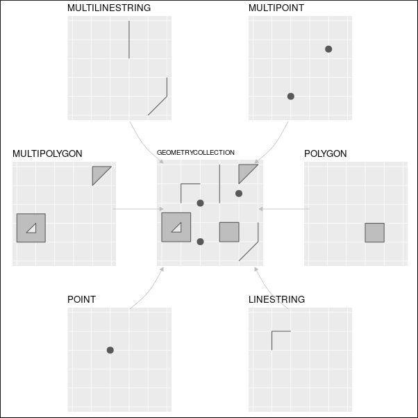
Simple features is a hierarchical data model that represents a wide range of geometry types. Of 18 geometry types supported by the specification, only seven are used in the vast majority of geographic research (see Figure 2.1); these core geometry types are fully supported by the R package {sf}.

---

Figure 2.1: Simple feature types fully supported by {sf}.

---

{sf} provides the same functionality (and more) previously provided in three (now deprecated) packages:

• {sp} for data classes
• {rgdal} for data read/write via an interface to GDAL and PROJ and
• {rgeos} for spatial operations via an interface to GEOS.

Note 2.1: Deprecated packages & the history of the R-spatial ecosystem

This detailed infos (together with the history of the R-spatial ecosystem provided in Chapter 1 of the book) I would have needed earlier. When I started to learn spatial data science (one month ago, December 2024) I was confused about the many different packages with similar functionality.

Resource 2.1 : {sf} documentation

sf’s functionality is well documented on its website at r-spatial.github.io/sf/ which contains seven vignettes.

1. Simple Features for R
2. Reading, Writing and Converting Simple Features
3. Manipulating Simple Feature Geometries
4. Manipulating Simple Features
5. Plotting Simple Features
6. Miscellaneous
7. Spherical geometry in sf using s2geometry

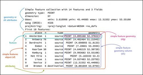
Simple feature objects in R are stored in a data frame, with geographic data occupying a special column, usually named ‘geom’ or ‘geometry’. Simple features are, in essence, data frames with a spatial extension.

Code Collection 2.1 : Inspect {sf} classes, plotting, summary, and subsetting

Inspect data

R Code 2.2 : Inspect class and column names of world

utils::data("world", package = "spData")
base::class(world)
base::names(world)

#> [1] "sf"         "tbl_df"     "tbl"        "data.frame"
#>  [1] "iso_a2"    "name_long" "continent" "region_un" "subregion" "type"     
#>  [7] "area_km2"  "pop"       "lifeExp"   "gdpPercap" "geom"

---

The contents of the geom column give {sf} objects their spatial powers: world$geom is a ‘list column’ that contains all the coordinates of the country polygons.

Plot data

R Code 2.3 : Plot world data

sf:::plot.sf(world) # plot produces only the first 9 attributes (1)

#> Warning: plotting the first 9 out of 10 attributes; use max.plot = 10 to plot
#> all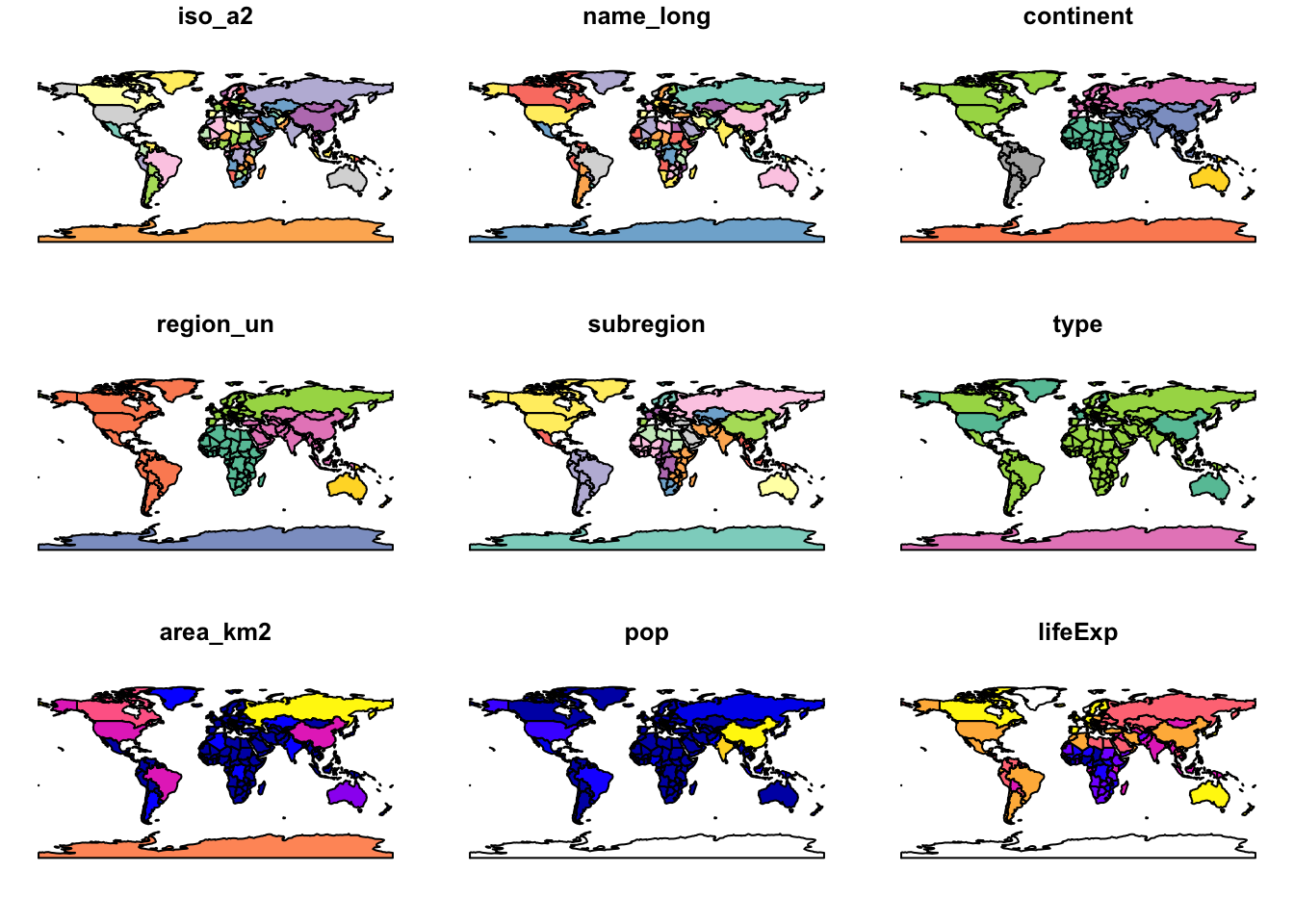

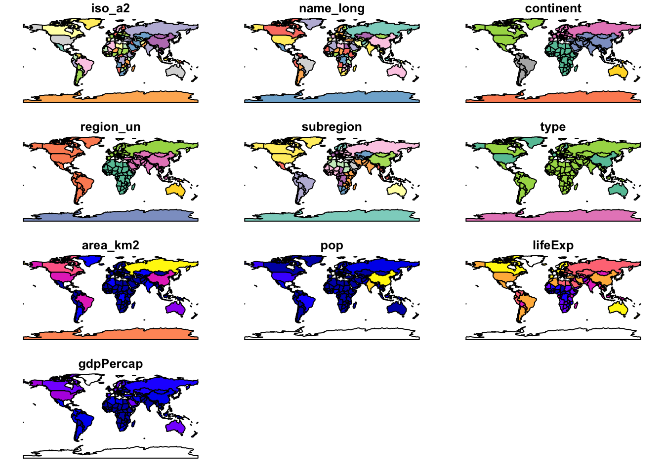
sf:::plot.sf(world, max.plot = 10) # 11 cols but 'geom' does not count as attribute (2)
sf:::plot.sf(world, max.plot = Inf) # plot all availabe attributes (3)

Figure 2.2: Map of the world using the {sf} package, with a facet for each attribute.

Figure 2.3: Map of the world using the {sf} package, with a facet for each attribute.

---

Instead of creating a single map by default for geographic objects, as most GIS programs do, plot()ing sf objects results in a map for each variable in the datasets. This behavior can be useful for exploring the spatial distribution of different variables.

If you attach the {sf} package with library(sf) then plot(world) would have worked. But it is not the base::plot() function as errors in line 2 and 3 would show. plot() is a generic function that is extended by other packages. {sf} contains the non-exported (hidden from users most of the time and therefore with three columns prefixed) sf:::plot.sf() function which is called behind the scenes.

Summary

R Code 2.4 : Treating sf objects as data frames

base::summary(world["lifeExp"]) # infos about the 'geom' column 

#>     lifeExp                 geom    
#>  Min.   :50.62   MULTIPOLYGON :177  
#>  1st Qu.:64.96   epsg:4326    :  0  
#>  Median :72.87   +proj=long...:  0  
#>  Mean   :70.85                      
#>  3rd Qu.:76.78                      
#>  Max.   :83.59                      
#>  NA's   :10

base::summary(world$lifeExp) # no infos about the 'geom' column

#>    Min. 1st Qu.  Median    Mean 3rd Qu.    Max.    NA's 
#>   50.62   64.96   72.87   70.85   76.78   83.59      10

---

Treating geographic objects as regular data frames with spatial powers has many advantages, especially if you are already used to working with data frames. The commonly used summary() function, for example, provides a useful overview of the variables within the world object.

Subsetting

R Code 2.5 : Subsetting sf object with base R and {dplyr}

world[1:2, 1:3] # base R subsetting

#> Simple feature collection with 2 features and 3 fields
#> Geometry type: MULTIPOLYGON
#> Dimension:     XY
#> Bounding box:  xmin: -180 ymin: -18.28799 xmax: 180 ymax: -0.95
#> Geodetic CRS:  WGS 84
#>   iso_a2 name_long continent                           geom
#> 1     FJ      Fiji   Oceania MULTIPOLYGON (((-180 -16.55...
#> 2     TZ  Tanzania    Africa MULTIPOLYGON (((33.90371 -0...

world |> # tidyverse subsetting
    dplyr::slice(1:2) |>
    dplyr::select(1:3)

#> Simple feature collection with 2 features and 3 fields
#> Geometry type: MULTIPOLYGON
#> Dimension:     XY
#> Bounding box:  xmin: -180 ymin: -18.28799 xmax: 180 ymax: -0.95
#> Geodetic CRS:  WGS 84
#> # A tibble: 2 × 4
#>   iso_a2 name_long continent                                                geom
#>   <chr>  <chr>     <chr>                                      <MULTIPOLYGON [°]>
#> 1 FJ     Fiji      Oceania   (((-180 -16.55522, -179.9174 -16.50178, -179.7933 …
#> 2 TZ     Tanzania  Africa    (((33.90371 -0.95, 31.86617 -1.02736, 30.76986 -1.…

---

Subsetting is another example where sf objects are treating as normal data frames. The output shows two major differences compared with a regular data.frame:

• the inclusion of additional geographic metadata (Geometry type, Dimension, Bounding box and coordinate reference system information), and
• the presence of a ‘geometry column’, here named “geom”.

Base R and tidyverse subsetting yield the same result, but with slightly different formatting of the ‘geom’ column.

Class of ‘geom’ column

R Code 2.6 : Class of the ‘geom’ column and of one entry of the ‘geom’ column

base::class(world) # class of sf object (sf)
base::class(world$geom) # class of 'geom' column (sfc)
base::class(world$geom[[1]]) # class of first entry of 'geom' (sfg)

#> [1] "sf"         "tbl_df"     "tbl"        "data.frame"
#> [1] "sfc_MULTIPOLYGON" "sfc"             
#> [1] "XY"           "MULTIPOLYGON" "sfg"

---

Here you can see the hierarchy of the three object types in the {sf} universe. I explain it in reverse order, starting with the lowest level:

• sfg (Simple Feature Gemometry) is the lowest unit; it has only coordinates (according to the well-known text (WKT) standard)
• sfc (Simple Feature Gemometry Collection) is a set of sfg’s, plus - crucially! - information about interpretation of the coordinate reference system / are the coordinates in meters, or degrees? plane or sphere? if sphere, which one? this is highly standardized stuff, often described in terms of EPSG codes (EPSG Geodetic Parameter Dataset).
• sf (Simple Feature) is a sfc geometry with data columns, in addition to the geometry.

2.2.2 Why simple features?

Simple features is a widely supported data model that underlies data structures in many GIS applications including QGIS and PostGIS.

There are numerous advantages using the {sf} package:

• Fast reading and writing of data
• Enhanced plotting performance
• sf objects can be treated as data frames in most operations
• sf function names are relatively consistent and intuitive (all begin with st_)
• sf functions can be combined with the |> operator and works well with the {tidyverse} collection of R packages.

sf::st_read() vs. sf::read_sf() are good examples to show and compare the support for the {tidyverse} pckages.

• sf::st_read() emits verbose messages and returns the file content stored in a base R data.frame.
• sf::read_sf() silently returns data as a tidyverse tibble.

R Code 2.7 : Compare sf::st_read() with sf::read_sf()

world_dfr = sf::st_read(system.file("shapes/world.gpkg", package = "spData"))

#> Reading layer `world' from data source 
#>   `/Library/Frameworks/R.framework/Versions/4.4-x86_64/Resources/library/spData/shapes/world.gpkg' 
#>   using driver `GPKG'
#> Simple feature collection with 177 features and 10 fields
#> Geometry type: MULTIPOLYGON
#> Dimension:     XY
#> Bounding box:  xmin: -180 ymin: -89.9 xmax: 180 ymax: 83.64513
#> Geodetic CRS:  WGS 84

world_tbl = sf::read_sf(system.file("shapes/world.gpkg", package = "spData"))
base::class(world_dfr) # base data.frame

#> [1] "sf"         "data.frame"

base::class(world_tbl) # tidyverse tibble

#> [1] "sf"         "tbl_df"     "tbl"        "data.frame"

---

Data files from the {spData} package are located in the folder “shapes” inside the {spData} package folder.This can be detected manually in the operating systems by opening the folder “spData” for the {spData} package. To get the file path one has to use the base::system.file() function with the appropriate package name and providing the path to the file inside this package: system.file("shapes/world.gpkg", package = "spData").

Note 2.2: {sf} is now the go-to package for analysis of spatial vector data in R

{spatstat}, a package ecosystem which provides numerous functions for spatial statistics, and {terra} both have vector geographic data classes, but neither has the same level of uptake as {sf} does for working with vector data. Many popular packages build on {sf}.

2.2.3 Basic Maps

Code Collection 2.2 : Basic maps created with {sf}

Multi-panel plot

R Code 2.8 : Multi-panel plot with {sf}

sf:::plot.sf(world[3:6])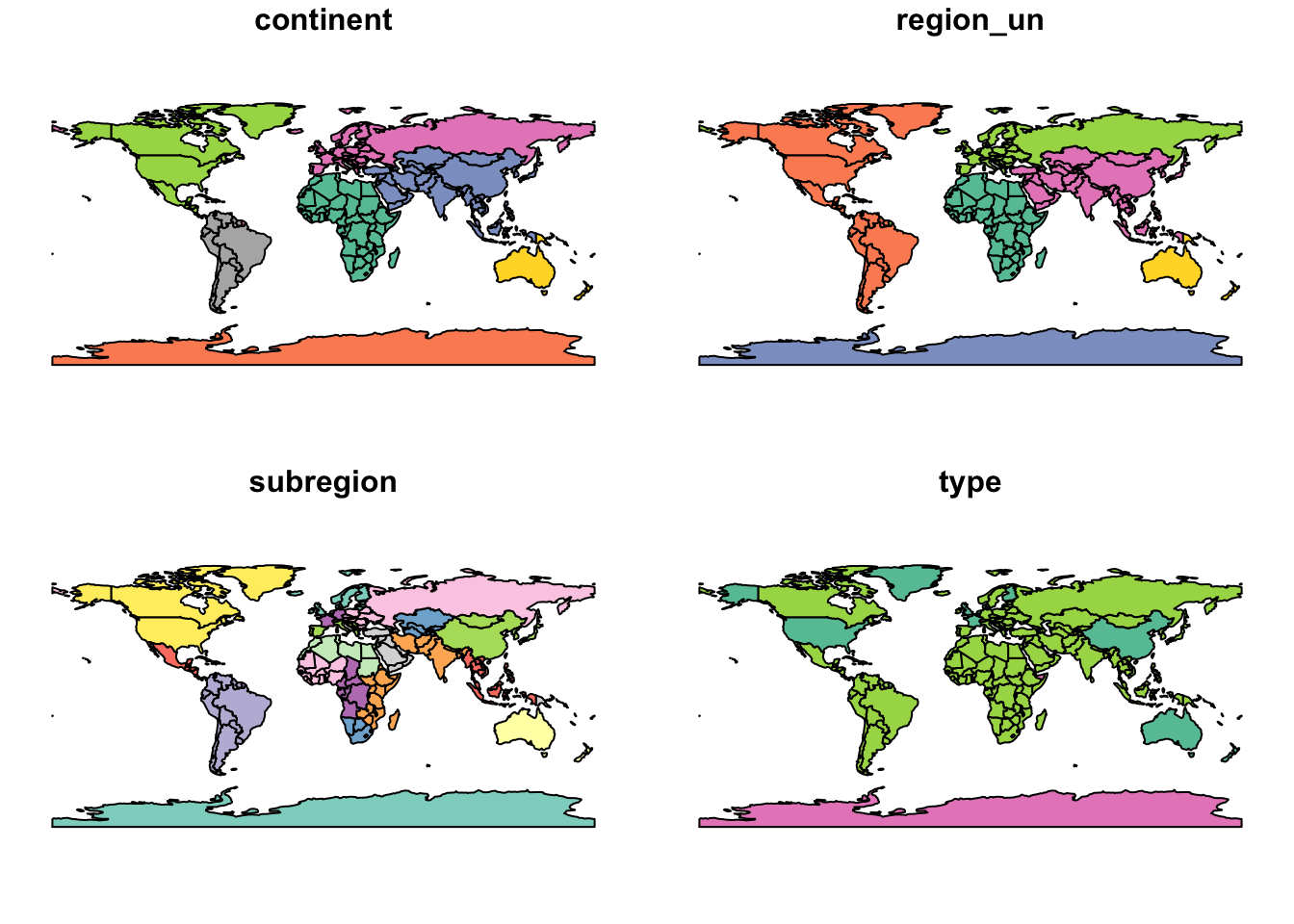

Figure 2.4: A multi-panel plot with {sf} creates one sub-plot for each variable of the object.

Single plot

R Code 2.9 : Single plot with {sf}

sf:::plot.sf(world["pop"])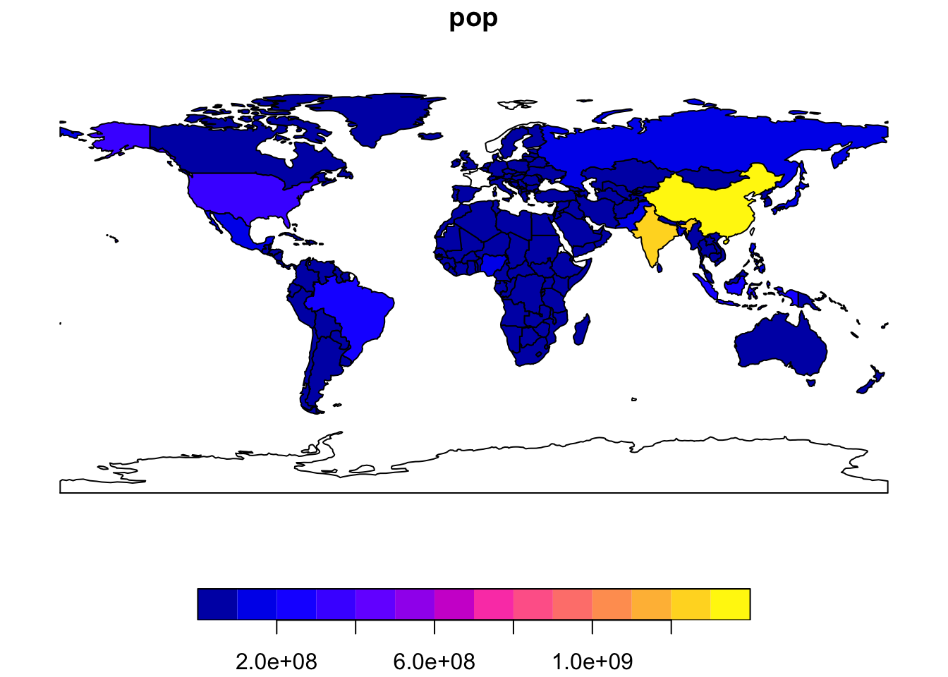

Figure 2.5: If the object to be plotted with {sf} has a single variable, then a legend with a continuous color is produced.

Fixed colors

R Code 2.10 : Plot with {sf} with fixed country and border colors

sf:::plot.sf(world["pop"], col = "lightblue", border = "black")

Figure 2.6: You can set fixed colors in the sf::plot.sf() commands with col and border arguments.

There are various ways to modify maps with {sf}’s plot() method. Because {sf} extends base R plotting methods, graphics::plot()’s arguments work with {sf} objects (see ?graphics::plot and ?par for information on arguments.)

Code Collection 2.3 : Adding different layers to plot output of sf objects

filters & combining

R Code 2.11 : Numbered R Code Title

utils::data("world", package = "spData") # get world data

base::library(sf) |> base::suppressPackageStartupMessages() # load {sf}

asia <-  world |> 
    dplyr::filter(continent == "Asia") |> # (1)
    sf::st_union()

plot(world["pop"], reset = FALSE)
plot(asia, add = TRUE, col = "red")

detach("package:sf", unload = TRUE) # return to previous state, unload {sf}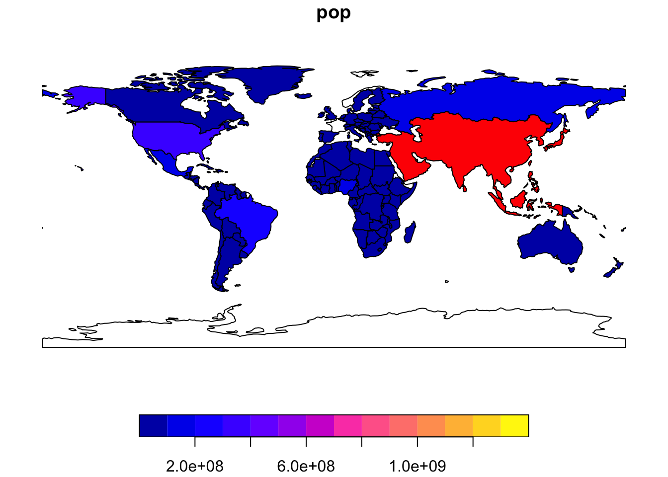

Figure 2.7: Plot of Asia added as a layer on top of countries worldwide.

---

Plots are added as layers to existing images by setting add = TRUE. Line (1) in the above code chunk filters countries in Asia and combines them in line (2) into a single feature.

We can now plot the Asian continent over a map of the world. Note that the first plot (line (3)) must only have one facet for add = TRUE to work. If the first plot has a key (legend), reset = FALSE must be used.

unprojected

R Code 2.12 : Overlay circles representing country population on a world map (unprojected version)

base::library(sf) |> base::suppressPackageStartupMessages() # load {sf}

plot(world["continent"], reset = FALSE)                    # (1)
cex = base::sqrt(world$pop) / 10000                        # (2)
world_cents = sf::st_centroid(world, of_largest = TRUE)    # (3)

#> Warning: st_centroid assumes attributes are constant over geometries

plot(sf::st_geometry(world_cents), add = TRUE, cex = cex)  # (4)

detach("package:sf", unload = TRUE) # return to previous state, unload {sf}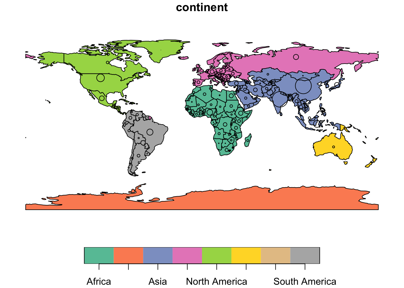

Figure 2.8: Overlaying circles, whose diameters (set with cex =) represent country populations, on a map of the world. Unprojected version

---

The code above uses the function sf::st_centroid() to convert one geometry type (polygons) to another (points) (see (XXXChapter5?)), the aesthetics of which are varied with the cex argument.

The sf::st_centroid() function (line 3) produced: ‘Warning: st_centroid assumes attributes are constant over geometries’.

“The reason for this is that the dataset contains variables with values that are associated with entire polygons … meaning they are not associated with a POINT geometry replacing the polygon.” (Pebesma and Bivand 2023, chap. 5)

projected

R Code 2.13 : Overlay circles representing country population on a world map (projected version)

utils::data("world", package = "spData")

base::library(sf) |> base::suppressPackageStartupMessages() # load {sf}

world_proj = sf::st_transform(world, "+proj=eck4")                                   # (1)
world_cents = sf::st_centroid(world_proj, of_largest_polygon = TRUE)                 # (2)

#> Warning: st_centroid assumes attributes are constant over geometries

graphics::par(mar = c(0, 0, 0, 0))                                                   # (3)
plot(world_proj["continent"], reset = FALSE, main = "", key.pos = NULL)              # (4)
g = sf::st_graticule()                                                               # (5)
g = sf::st_transform(g, crs = "+proj=eck4")                                          # (6)
plot(g$geometry, add = TRUE, col = "lightgray")                                      # (7)
cex = base::sqrt(world$pop) / 10000                                                  # (8)
plot(sf::st_geometry(world_cents), add = TRUE, cex = cex, lwd = 2, graticule = TRUE) # (9)

detach("package:sf", unload = TRUE) # return to previous state, unload {sf}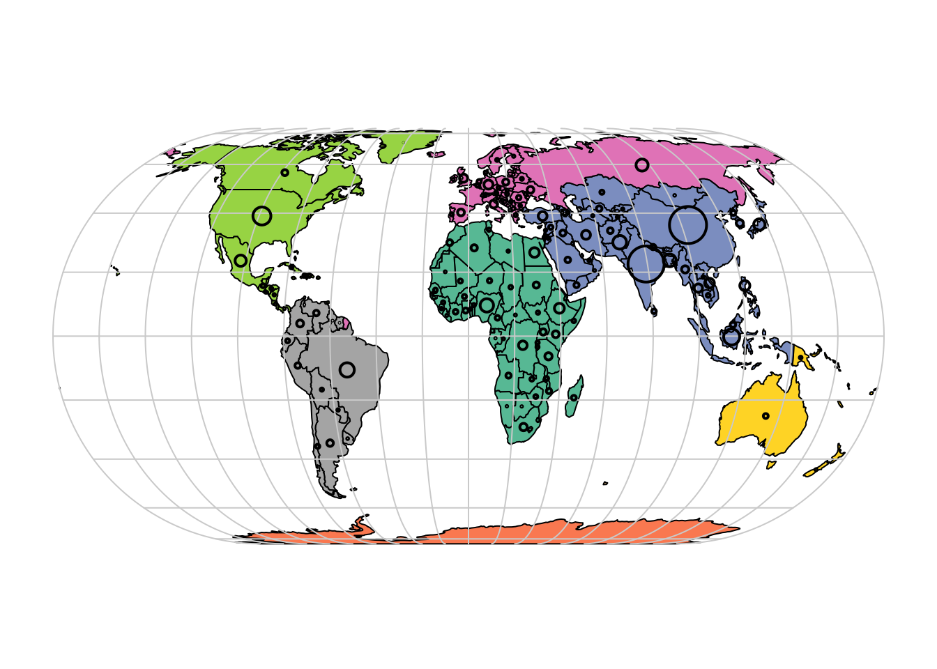

Figure 2.9: Overlaying circles, whose diameters (set with cex =) represent country populations, on a map of the world. Projected version

---

For the above code I used the script 02-contplot.R. There are new code lines to change the unprojected to a projected figure that I do not yet understand fully.

In all code chunks of this code collection I had to attach {sf} because the sf:plot.sf() commands did not work. I received the error message ‘Error in if (ncol(x) == 1) { : argument is of length zero’. After changing the original code of the function to if (isTRUE(x) && ncol(x) == 1) I received other errors. Finally I gave up and used the standard base::library(sf).

{sf}’s plot method also has arguments specific to geographic data. expandBB, for example, can be used to plot an sf object in context: it takes a numeric vector of length four that expands the bounding box of the plot relative to zero in the following order: bottom, left, top, right. This is used in the following code to plot India in the context of its giant Asian neighbors, with an emphasis on China to the east.

Code Collection 2.4 : Using expandBB argument to plot an sf object in context

no labels

R Code 2.14 : Creating context by plotting with the expandBB argument (without labels)

base::library(sf) |> base::suppressPackageStartupMessages() # load {sf}

india <- world |> 
    dplyr::filter(name_long == "India")
world_asia <- world |> 
    dplyr::filter(continent == "Asia")

plot(sf::st_geometry(india), expandBB = c(-0.2, 0.5, 0, 1), col = "gray", lwd = 3)
plot(sf::st_geometry(world_asia), add = TRUE)

detach("package:sf", unload = TRUE) # return to previous state, unload {sf}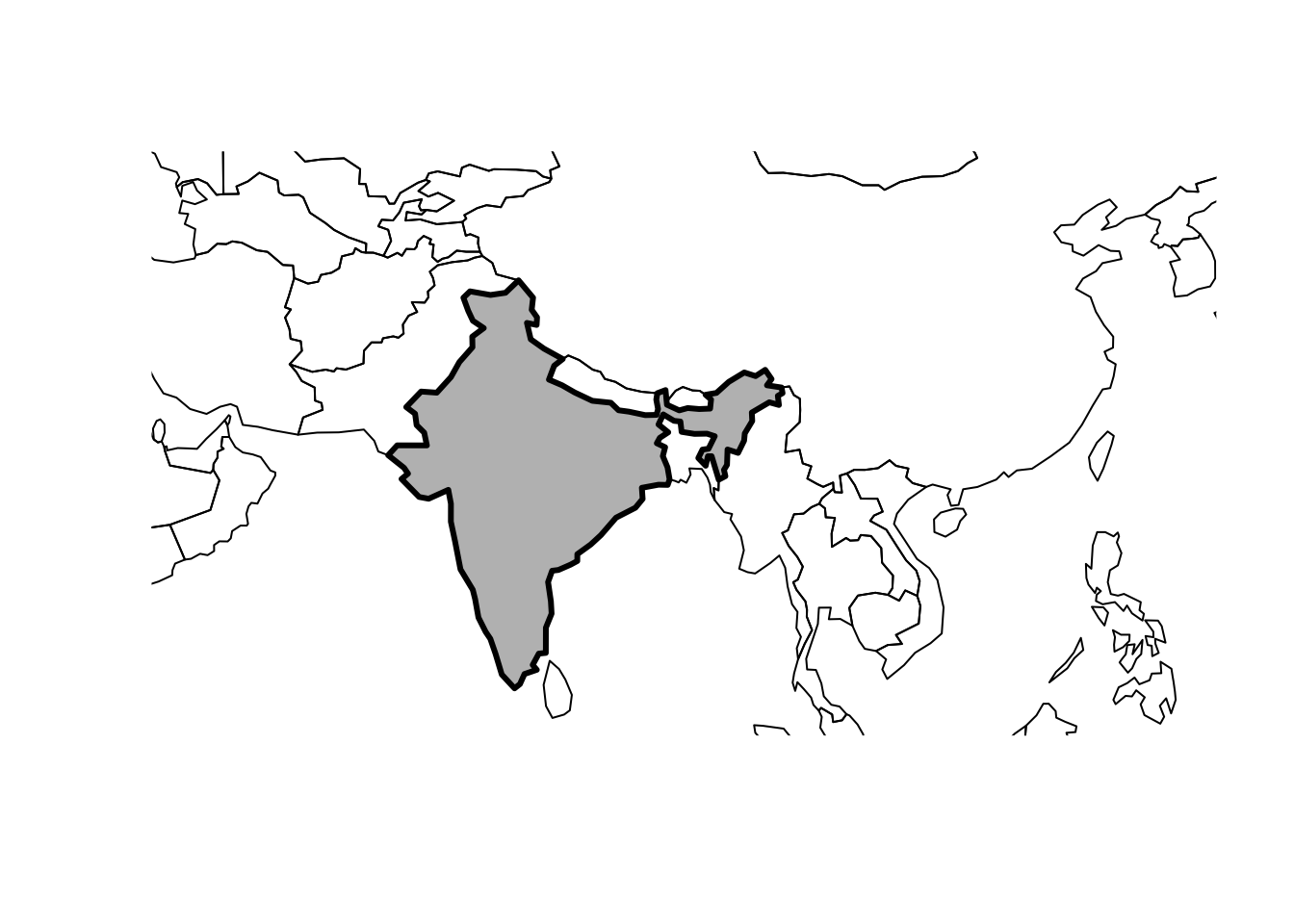

Figure 2.10: India in context, demonstrating the expandBB argument (without labels).

with labels

R Code 2.15 : Creating context by plotting with the expandBB argument (with labels)

utils::data("world", package = "spData")
base::library(sf) |> base::suppressPackageStartupMessages() # load {sf}

india <- world |> 
    dplyr::filter(name_long == "India")
world_asia <- world |> 
    dplyr::filter(continent == "Asia")
indchi  <-  
    world_asia[grepl("Indi|Chi", world_asia$name_long), ]
indchi_coords <- 
    sf::st_centroid(indchi) |> 
    sf::st_coordinates()

old_par = graphics::par(mar = rep(0, 4))

plot(sf::st_geometry(india), expandBB = c(-0.2, 0.5, 0, 1), col = "gray", lwd = 3)
plot(world_asia[0], add = TRUE)
terra::text(indchi_coords[, 1], indchi_coords[, 2], indchi$name_long)

graphics::par(old_par)

detach("package:sf", unload = TRUE) # return to previous state, unload {sf}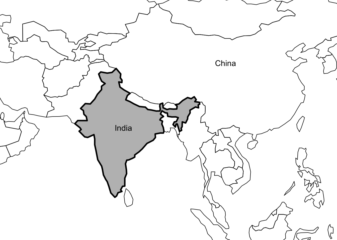

Figure 2.11: India in context, demonstrating the expandBB argument (with labels).

Note the use of lwd (linewidth) to emphasize India in the plotting code. See (XXXChapter9-2?) for other visualization techniques for representing a range of geometry types, the subject of the next section.

2.2.4 Geometry types

Generally, well-known binary (WKB) or well-known text (WKT) are the standard encoding for simple feature geometries.

• WKB representations are usually hexadecimal strings easily readable for computers. This is why GIS and spatial databases use WKB to transfer and store geometry objects.
• WKT, on the other hand, is a human-readable text markup description of simple features. Both formats are exchangeable.

2.2.5 The sf class

Simple features consist of two main parts: geometries and non-geographic attributes. Figure 2.12 shows how an sf object is created – geometries come from an sfc object, while attributes are taken from a data.frame or tibble.

Figure 2.12: Building blocks of sf objects

More about building sf geometries from scratch see Section 2.2.6 and Section 2.2.7.

Code Collection 2.5 : Creation and Class of sf Building Blocks

Creation

R Code 2.16 : Building blocks of sf objects

(lnd_point = sf::st_point(c(0.1, 51.5))   )              # (1) sfg object

#> POINT (0.1 51.5)

(lnd_geom = sf::st_sfc(lnd_point, crs = "EPSG:4326"))    # (2) sfc object

#> Geometry set for 1 feature 
#> Geometry type: POINT
#> Dimension:     XY
#> Bounding box:  xmin: 0.1 ymin: 51.5 xmax: 0.1 ymax: 51.5
#> Geodetic CRS:  WGS 84

#> POINT (0.1 51.5)

(
    lnd_attrib = base::data.frame(                       # (3) data.frame object
      name = "London",
      temperature = 25,
      date = base::as.Date("2023-06-21")
    )
)

#>     name temperature       date
#> 1 London          25 2023-06-21

(lnd_sf = sf::st_sf(lnd_attrib, geometry = lnd_geom))    # (4) sf object

#> Simple feature collection with 1 feature and 3 fields
#> Geometry type: POINT
#> Dimension:     XY
#> Bounding box:  xmin: 0.1 ymin: 51.5 xmax: 0.1 ymax: 51.5
#> Geodetic CRS:  WGS 84
#>     name temperature       date         geometry
#> 1 London          25 2023-06-21 POINT (0.1 51.5)

---

• Line 1: The coordinates were used to create the simple feature geometry (sfg).
• Line 2: The geometry was converted into a simple feature geometry column (sfc), with a CRS.
• Line 3: Attributes were stored in a data.frame.
• Line 4: The data.frame was combined with the sfc object. The results in an sf object.

The result shows that sf objects actually have two classes, sf and data.frame. Simple features are simply data frames (square tables), but with spatial attributes stored in a list column, usually called geometry or geom. This duality is central to the concept of simple features: most of the time a sf can be treated as and behaves like a data.frame. Simple features are, in essence, data frames with a spatial extension.

Classes

R Code 2.17 : Classes of sf Building Blocks

base::class(lnd_point)  # sfg

#> [1] "XY"    "POINT" "sfg"

base::class(lnd_geom)   # sfc

#> [1] "sfc_POINT" "sfc"

base::class(lnd_attrib) # data.frame

#> [1] "data.frame"

base::class(lnd_sf)     # sf

#> [1] "sf"         "data.frame"

---

Depending of the created geometry type POINT can be replaced by LINESTRING, POLYGON, MUTLIPOINT, MULTILINESTRING, MULTIPOLYGON. It is most often the case that the objects are of identical type. In case of a mix of types or an empty set, POINT (or any of the other mentioned gemoetries) are set to the superclass GEOMETRY.

Figure 2.13 shows — as a kind of summary — the different sf objects in their contexts (Picture taken from Sadler 2018).

Figure 2.13: Building Blocks of sf objects

2.2.6 Simple feature geometries (sfg)

The sfg class represents the different simple feature geometry types in R: point, linestring, polygon (and their ‘multi’ equivalents, such as multipoints) or geometry collection.

Usually you are spared the tedious task of creating geometries on your own since you can simply import an already existing spatial file. However, there are a set of functions to create simple feature geometry objects (sfg) from scratch, if needed. The names of these functions are simple and consistent, as they all start with the st_ prefix and end with the name of the geometry type in lowercase letters:

• A point: sf::st_point()
• A linestring: sf::st_linestring()
• A polygon: sf::st_polygon()
• A multipoint: sf::st_multipoint()
• A multilinestring: sf::st_multilinestring()
• A multipolygon: sf::st_multipolygon()
• A geometry collection: sf::st_geometrycollection()

sfg objects can be created from three base R data types:

• Numeric vector: a single point
• Matrix: a set of points, where each row represents a point, a multipoint or linestring
• List: a collection of objects such as matrices, multilinestrings or geometry collections.

Code Collection 2.6 : Creating Simple Feature Geometries (sfg)

Numeric Vectors

R Code 2.18 : Create single points from numerical vectors

sf::st_point(base::c(5, 2))                 # XY point

#> POINT (5 2)

sf::st_point(base::c(5, 2, 3))              # XYZ point

#> POINT Z (5 2 3)

sf::st_point(base::c(5, 2, 1), dim = "XYM") # XYM point

#> POINT M (5 2 1)

sf::st_point(base::c(5, 2, 3, 1))           # XYZM point

#> POINT ZM (5 2 3 1)

---

“XYZ” refers to coordinates where the third dimension represents altitude, “XYM” refers to three-dimensional coordinates where the third dimension refers to something else (“M” for measure).

The results show that XY (2D coordinates), XYZ (3D coordinates, Z = altitude) and XYZM (3D with an additional variable, typically measurement accuracy, M = measurement) point types are created from vectors of lengths 2, 3, and 4, respectively. The XYM type must be specified using the dim argument (which is short for dimension).

Matrices

R Code 2.19 : Create multipoint and linestring from matrices

multipoint_matrix = base::rbind(c(5, 2), c(1, 3), c(3, 4), c(3, 2))
sf::st_multipoint(multipoint_matrix) ## MULTIPOINT

#> MULTIPOINT ((5 2), (1 3), (3 4), (3 2))

linestring_matrix = base::rbind(c(1, 5), c(4, 4), c(4, 1), c(2, 2), c(3, 2))
sf::st_linestring(linestring_matrix) ## LINESTRING

#> LINESTRING (1 5, 4 4, 4 1, 2 2, 3 2)

---

The base::rbind() function simplifies the creation of matrices.

I have base:: not prefixed to c().

Lists

R Code 2.20 : Create polygons from lists

## POLYGON
polygon_list = base::list(base::rbind(c(1, 5), c(2, 2), c(4, 1), c(4, 4), c(1, 5)))
sf::st_polygon(polygon_list) 

#> POLYGON ((1 5, 2 2, 4 1, 4 4, 1 5))

## POLYGON with a hole
polygon_border = base::rbind(c(1, 5), c(2, 2), c(4, 1), c(4, 4), c(1, 5))
polygon_hole = base::rbind(c(2, 4), c(3, 4), c(3, 3), c(2, 3), c(2, 4))
polygon_with_hole_list = base::list(polygon_border, polygon_hole)
sf::st_polygon(polygon_with_hole_list) 

#> POLYGON ((1 5, 2 2, 4 1, 4 4, 1 5), (2 4, 3 4, 3 3, 2 3, 2 4))

## MULTILINESTRING
multilinestring_list = base::list(base::rbind(c(1, 5), c(4, 4), c(4, 1), c(2, 2), c(3, 2)), 
                            base::rbind(c(1, 2), c(2, 4)))
sf::st_multilinestring(multilinestring_list) 

#> MULTILINESTRING ((1 5, 4 4, 4 1, 2 2, 3 2), (1 2, 2 4))

## MULTIPOLYGON
multipolygon_list = base::list(base::list(base::rbind(c(1, 5), c(2, 2), c(4, 1), c(4, 4), c(1, 5))),
                         base::list(base::rbind(c(0, 2), c(1, 2), c(1, 3), c(0, 3), c(0, 2))))
sf::st_multipolygon(multipolygon_list) 

#> MULTIPOLYGON (((1 5, 2 2, 4 1, 4 4, 1 5)), ((0 2, 1 2, 1 3, 0 3, 0 2)))

## GEOMETRYCOLLECTION
geometrycollection_list = base::list(sf::st_multipoint(multipoint_matrix),
                              sf::st_linestring(linestring_matrix))
sf::st_geometrycollection(geometrycollection_list) 

#> GEOMETRYCOLLECTION (MULTIPOINT ((5 2), (1 3), (3 4), (3 2)), LINESTRING (1 5, 4 4, 4 1, 2 2, 3 2))

---

I have base:: not prefixed to c().

2.2.7 Simple feature columns (sfc)

One sfg object contains only a single simple feature geometry. A simple feature geometry column (sfc) is a list of sfg objects, which is additionally able to contain information about the CRS in use. For instance, to combine two simple features into one object with two features, we can use the sf::st_sfc() function. This is important since sfc represents the geometry column in sf data frames.

Code Collection 2.7 : Simple feature columns (sfc)

sfc POINT

R Code 2.21 : Geometry set of two POINTS features

point1 = sf::st_point(c(5, 2))
point2 = sf::st_point(c(1, 3))
points_sfc = sf::st_sfc(point1, point2)
points_sfc

#> Geometry set for 2 features 
#> Geometry type: POINT
#> Dimension:     XY
#> Bounding box:  xmin: 1 ymin: 2 xmax: 5 ymax: 3
#> CRS:           NA

#> POINT (5 2)

#> POINT (1 3)

---

Besides returning the dimensions of the bounding box it also returns the CRS. In this case it is NA (not available)

sfc POLYGON

R Code 2.22 : Geometry set of two POLYGON features and showing the resulting sfc types

polygon_list1 = list(rbind(c(1, 5), c(2, 2), c(4, 1), c(4, 4), c(1, 5)))
polygon1 = sf::st_polygon(polygon_list1)
polygon_list2 = list(rbind(c(0, 2), c(1, 2), c(1, 3), c(0, 3), c(0, 2)))
polygon2 = sf::st_polygon(polygon_list2)
( polygon_sfc = sf::st_sfc(polygon1, polygon2) )

#> Geometry set for 2 features 
#> Geometry type: POLYGON
#> Dimension:     XY
#> Bounding box:  xmin: 0 ymin: 1 xmax: 4 ymax: 5
#> CRS:           NA

#> POLYGON ((1 5, 2 2, 4 1, 4 4, 1 5))

#> POLYGON ((0 2, 1 2, 1 3, 0 3, 0 2))

( geom_type <- sf::st_geometry_type(polygon_sfc) )

#> [1] POLYGON POLYGON
#> 18 Levels: GEOMETRY POINT LINESTRING POLYGON MULTIPOINT ... TRIANGLE

base::class(polygon_sfc)

#> [1] "sfc_POLYGON" "sfc"

base::class(geom_type)

#> [1] "factor"

base::levels(geom_type)

#>  [1] "GEOMETRY"           "POINT"              "LINESTRING"        
#>  [4] "POLYGON"            "MULTIPOINT"         "MULTILINESTRING"   
#>  [7] "MULTIPOLYGON"       "GEOMETRYCOLLECTION" "CIRCULARSTRING"    
#> [10] "COMPOUNDCURVE"      "CURVEPOLYGON"       "MULTICURVE"        
#> [13] "MULTISURFACE"       "CURVE"              "SURFACE"           
#> [16] "POLYHEDRALSURFACE"  "TIN"                "TRIANGLE"

---

In most cases, an sfc object contains objects of the same geometry type. Therefore, when we convert sfg objects of type polygon into a simple feature geometry column, we would also end up with an sfc object of type polygon, which can be verified with sf::st_geometry_type().

(You will get a similar result binding several MULTILINESTRINGs together, or another type of geometry. I will skip this code chunk.)

Additionally I was here interested to get all 18 levels of the geometry type of “polygon_sfc” with base::levels(). I knew already of the first eight but the rest are new to me. Detailed information about all types can be found in the {sf} vignette 1. Simple Features of R under the section Simple feature geometry types.

Note 2.3: What is the difference between GEOMETRY and GEOMETRYCOLLECTION?

• GEOMETRY is used to describe a list of geometries of varying types or an empty set.
• GEOMETRYCOLLECTION is used to describe a single geometry that can contain multiple types of geometries.

(Here I have abstained from prefixing base:: to c(), list() and rbind())

sfc GEOMETRY

R Code 2.23 : Geometry set of two different geometry features and showing the resulting sfc types

point_polygon_sfc = sf::st_sfc(point1, polygon1) 
sf::st_geometry_type(point_polygon_sfc)

#> [1] POINT   POLYGON
#> 18 Levels: GEOMETRY POINT LINESTRING POLYGON MULTIPOINT ... TRIANGLE

class(point_polygon_sfc)

#> [1] "sfc_GEOMETRY" "sfc"

---

It is also possible to create an sfc object from sfg objects with different geometry types. It results in the superclass GEOMETRY.

Set CRS

R Code 2.24 : Check and set Coordinate Reference System (CRS)

# Check the CRS
sf::st_crs(points_sfc)

#> Coordinate Reference System: NA

# Set the CRS with an identifier referring to an 'EPSG' CRS code:
points_sfc_wgs = sf::st_sfc(point1, point2, crs = "EPSG:4326")

# print CRS
sf::st_crs(points_sfc_wgs) 

#> Coordinate Reference System:
#>   User input: EPSG:4326 
#>   wkt:
#> GEOGCRS["WGS 84",
#>     ENSEMBLE["World Geodetic System 1984 ensemble",
#>         MEMBER["World Geodetic System 1984 (Transit)"],
#>         MEMBER["World Geodetic System 1984 (G730)"],
#>         MEMBER["World Geodetic System 1984 (G873)"],
#>         MEMBER["World Geodetic System 1984 (G1150)"],
#>         MEMBER["World Geodetic System 1984 (G1674)"],
#>         MEMBER["World Geodetic System 1984 (G1762)"],
#>         MEMBER["World Geodetic System 1984 (G2139)"],
#>         ELLIPSOID["WGS 84",6378137,298.257223563,
#>             LENGTHUNIT["metre",1]],
#>         ENSEMBLEACCURACY[2.0]],
#>     PRIMEM["Greenwich",0,
#>         ANGLEUNIT["degree",0.0174532925199433]],
#>     CS[ellipsoidal,2],
#>         AXIS["geodetic latitude (Lat)",north,
#>             ORDER[1],
#>             ANGLEUNIT["degree",0.0174532925199433]],
#>         AXIS["geodetic longitude (Lon)",east,
#>             ORDER[2],
#>             ANGLEUNIT["degree",0.0174532925199433]],
#>     USAGE[
#>         SCOPE["Horizontal component of 3D system."],
#>         AREA["World."],
#>         BBOX[-90,-180,90,180]],
#>     ID["EPSG",4326]]

---

All geometries in sfc objects must have the same CRS. A CRS can be specified with the crs argument of sf::st_sfc() (or sf::st_sf()), which takes a CRS identifier provided as a text string, such as crs = "EPSG:4326" (see (XXXSection7-2?) for other CRS representations and details on what this means).

2.2.8 The sfheaders package

{sfheaders} is an R package that speeds-up the construction, conversion and manipulation of sf objects (Cooley 2024)). It focuses on building sf objects from vectors, matrices and data frames, rapidly, and without depending on the {sf} library; and exposing its underlying C++ code through header files (hence the name, sfheaders). (See the package profile at Section A.3.)

This approach enables others to extend it using compiled and fast-running code. Every core {sfheaders} function has a corresponding C++ implementation, as described in the Cpp vignette. For most people, the R functions will be more than sufficient to benefit from the computational speed of the package. {sfheaders} was developed separately from {sf}, but aims to be fully compatible, creating valid sf objects of the type described in preceding sections.

The simplest use case for sfheaders is demonstrated in the code chunks below with examples of building sfg, sfc, and sf objects showing:

• A vector converted to sfg_POINT
• A matrix converted to sfg_LINESTRING
• A data frame converted to sfg_POLYGON

Code Collection 2.8 : Title for code collection

Vector

R Code 2.25 : Creating the simplest possible sfg object

v = base::c(1, 1)
v_sfg_sfh = sfheaders::sfg_point(obj = v)
v_sfg_sfh # printing without sf loaded

#> POINT (1 1)

#>      [,1] [,2]
#> [1,]    1    1
#> attr(,"class")
#> [1] "XY"    "POINT" "sfg" 


# printing with sf loading
v_sfg_sf = sf::st_point(v)
base::print(v_sfg_sf) == print(v_sfg_sfh)

#> POINT (1 1)
#> POINT (1 1)

#> [1] TRUE

---

This creates the simplest possible sfg object, a single coordinate pair, assigned to a vector named v:

Instead to get as result the underlying structure from the first part of the code (it should result in the four lines of the out-commented code) I got just POINT (1 1). I do not know why this is the case. The version 0.4.4 from 2024-01-18 I have used here newer than the version in the book. Perhaps that the reason that the results are now identical between loading {sf} and not loading it?

When printing with {sf} loaded, my result is identical with the output in the book.

Matrix and data.frame

R Code 2.26 : Creating sfg objects from matrices and data frames with {sfheaders}

# matrices
m = base::matrix(1:8, ncol = 2)
sfheaders::sfg_linestring(obj = m)

#> LINESTRING (1 5, 2 6, 3 7, 4 8)

# data frames
df = base::data.frame(x = 1:4, y = 4:1)
sfheaders::sfg_polygon(obj = df)

#> POLYGON ((1 4, 2 3, 3 2, 4 1, 1 4))

---

sfc

R Code 2.27 : Creating simple feature columns (sfc) with {sfheaders}

sfheaders::sfc_point(obj = v)

#> Geometry set for 1 feature 
#> Geometry type: POINT
#> Dimension:     XY
#> Bounding box:  xmin: 1 ymin: 1 xmax: 1 ymax: 1
#> CRS:           NA

#> POINT (1 1)

sfheaders::sfc_linestring(obj = m)

#> Geometry set for 1 feature 
#> Geometry type: LINESTRING
#> Dimension:     XY
#> Bounding box:  xmin: 1 ymin: 5 xmax: 4 ymax: 8
#> CRS:           NA

#> LINESTRING (1 5, 2 6, 3 7, 4 8)

sfheaders::sfc_polygon(obj = df)

#> Geometry set for 1 feature 
#> Geometry type: POLYGON
#> Dimension:     XY
#> Bounding box:  xmin: 1 ymin: 1 xmax: 4 ymax: 4
#> CRS:           NA

#> POLYGON ((1 4, 2 3, 3 2, 4 1, 1 4))

sf

R Code 2.28 : Creating sf objects with {sfheaders}

sfheaders::sf_point(obj = v)

#> Simple feature collection with 1 feature and 0 fields
#> Geometry type: POINT
#> Dimension:     XY
#> Bounding box:  xmin: 1 ymin: 1 xmax: 1 ymax: 1
#> CRS:           NA
#>      geometry
#> 1 POINT (1 1)

sfheaders::sf_linestring(obj = m)

#> Simple feature collection with 1 feature and 1 field
#> Geometry type: LINESTRING
#> Dimension:     XY
#> Bounding box:  xmin: 1 ymin: 5 xmax: 4 ymax: 8
#> CRS:           NA
#>   id                       geometry
#> 1  1 LINESTRING (1 5, 2 6, 3 7, ...

sfheaders::sf_polygon(obj = df)

#> Simple feature collection with 1 feature and 1 field
#> Geometry type: POLYGON
#> Dimension:     XY
#> Bounding box:  xmin: 1 ymin: 1 xmax: 4 ymax: 4
#> CRS:           NA
#>   id                       geometry
#> 1  1 POLYGON ((1 4, 2 3, 3 2, 4 ...

CRS

R Code 2.29 : Setting the CRS for calculations or geometric operations using {sf} functions

df_sf = sfheaders::sf_polygon(obj = df)
sf::st_crs(df_sf) = "EPSG:4326"

In all of the previous examples of this code collection, the CRS was not defined. If you plan on doing any calculations or geometric operations using sf functions, we encourage you to set the CRS (see (XXXChapter7?) for details):

{sfheaders} is also good at ‘deconstructing’ and ‘reconstructing’ sf objects, meaning converting geometry columns into data frames that contain data on the coordinates of each vertex and geometry feature (and multi-feature) ids. It is fast and reliable at ‘casting’ geometry columns to different types, a topic covered in (XXXChapter5?). Benchmarks, in the package’s documentation show it is much faster than the {sf} package for such operations.

Remark 2.1. : {sfheaders} at the moment for me not relevant

I understand that the biggest advantage of {sfheaders} is speed in the calculation. At the moment I agree with the following observation:

For most people, the R functions [of the {sf} package] will be more than sufficient to benefit from the computational speed of the package.

Additionally I am still lacking experience with {sf} and therefore don’t want to learn similar packages at the same time.

2.2.9 Spherical geometry operations with S2

Since {sf} version 1.0.0, R supports spherical geometry operations ‘out of the box’ (and by default), thanks to its interface to Google’s S2 spherical geometry engine via the {s2} interface package (s2 package profile: Section A.1).

S2 is perhaps best known as an example of a Discrete Global Grid System (DGGS). Another example is the H3 global hexagonal hierarchical spatial index, supported by the R packages {h3r}, {h3jsr}, and {h3lib}. The differences is a complex theme I don’t want to tackle yet with my insufficient geocomputing knowledge.

Although potentially useful for describing locations anywhere on Earth using character strings, the main benefit of {sf}’s interface to {S2} is its provision of drop-in functions for calculations such as distance, buffer, and area calculations, as described in vignette 7 of {sf}’s documentation.

{sf} can run in two modes with respect to {S2}: on and off. By default the {S2} geometry engine is turned on, as can be verified with the following command: sf::sf_use_s2() results in TRUE.

An example of the consequences of turning the geometry engine off can be shown, by creating buffers around the india object created earlier in the chapter (note the warnings emitted when S2 is turned off):

R Code 2.30 : Example of the consequences of turning the geometry engine off

india_buffer_with_s2 = sf::st_buffer(india, 1) # 1 meter
sf::sf_use_s2(FALSE)

#> Spherical geometry (s2) switched off

india_buffer_without_s2 = sf::st_buffer(india, 1) # 1 degree

#> Warning in st_buffer.sfc(st_geometry(x), dist, nQuadSegs, endCapStyle =
#> endCapStyle, : st_buffer does not correctly buffer longitude/latitude data

#> dist is assumed to be in decimal degrees (arc_degrees).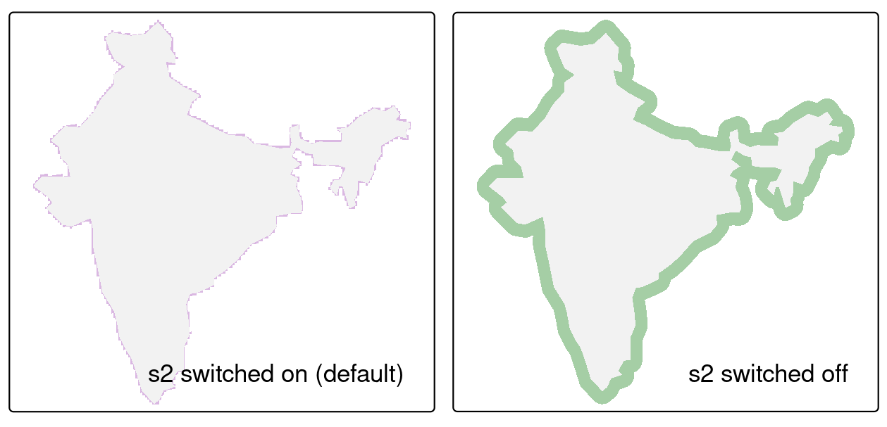

Figure 2.14: Example of the consequences of turning off the S2 geometry engine.

Both representations of a buffer around India were created with the same command sf::st_buffer(india, 1) but the purple polygon object was created with S2 switched on, resulting in a buffer of 1 m. The larger light green polygon was created with S2 switched off, resulting in a buffer of 1 degree, which is not accurate.

The right panel of Figure 2.12 is incorrect, as the buffer of 1 degree does not return the equal distance around the india polygon. (The explanation why this is the case comes in (XXXSection7-4?)).

Throughout this book, we will assume that S2 is turned on, unless explicitly stated. There some edge cases include operations on polygons that are not valid according to S2’s stricter definition. If you see error messages such as #> Error in s2_geography_from_wkb ... it may be worth trying the command that generated the error message again, after turning off S2.

R Code 2.31 : Turn S2 on again

sf::sf_use_s2(TRUE)
sf::sf_use_s2()

#> [1] TRUE

2.3 Raster data

The spatial raster data model represents the world with the continuous grid of cells (often also called pixels). It usually consists of a raster header and a matrix (with rows and columns) representing equally spaced cells. The raster header defines the CRS, the extent and the origin. The origin (or starting point) is frequently the coordinate of the lower left corner of the matrix (the {terra} package, however, uses the upper left corner, by default. The header defines the extent via the number of columns, the number of rows and the cell size resolution.

Starting from the origin, we can easily access and modify each single cell by either using the ID of a cell or by explicitly specifying the rows and columns. This and map algebra ((XXXSection4-3-2?)) make raster processing much more efficient and faster than vector data processing. In contrast to vector data, the cell of one raster layer can only hold a single value¹. The value might be continuous or categorical.

Raster maps usually represent continuous phenomena such as elevation, temperature, population density or spectral data. Discrete features such as soil or land-cover classes can also be represented in the raster data model. Depending on the nature of the application, vector representations of discrete features may be more suitable.

2.3.1 R packages for working with raster data

Most important nowadays is {terra}, which replaces the older {raster} and {stars}. This book focuses on {terra} but it is important to know the differences to {stars}:

• {terra} focuses on the most common raster data model (regular grids), while stars also allows storing less popular models (including regular, rotated, sheared, rectilinear, and curvilinear grids).

• {terra} usually handles one or multi-layered rasters, whereas {stars} provides ways to store raster data cubes – a raster object with many layers (e.g., bands), for many moments in time (e.g., months), and many attributes (e.g., sensor type A and sensor type B).

• In both packages all layers or elements of a data cube must have the same spatial dimensions and extent. Both packages allow to either read all of the raster data into memory or just to read its metadata – this is usually done automatically based on the input file size. However, they store raster values very differently.

• {terra} is based on C++ code and mostly uses C++ pointers whereas {stars} stores values as lists of arrays for smaller rasters or just a file path for larger ones.

• {terra} uses its own class of objects for vector data, namely SpatVector, but also accepts {sf} classes, whereas {stars} functions are closely related to the vector objects and functions in {sf}.

But it also possible to convert between these classes: terra::vect() from sf to SpatVector and sf::st_as_sf() from SpatVector to sf.

Fourth, both packages have a different approach for how various functions work on their objects.

• {terra} mostly relies on a large number of built-in functions, where each function has a specific purpose (e.g., resampling or cropping). On the other hand, {stars} uses some built-in functions (usually with names starting with st_), some existing {dplyr} functions (e.g., dplyr::filter() or dplyr::slice()), and also has its own methods for existing R functions (e.g., base::split() or or stats::aggregate()).

Importantly, it is straightforward to convert objects from {terra} to {stars} (using sf::st_as_stars()) and the other way round (using terra::rast()). We also encourage you to read (Pebesma and Bivand 2023) for the most comprehensive introduction to the {stars} package.

2.3.2 Introduction to {terra}

• The {terra} package supports raster objects in R. It provides an extensive set of functions to create, read, export, manipulate and process raster datasets.
• In addition to functions for raster data manipulation, {terra} provides many low-level functions that can form a foundation for developing new tools for working with raster datasets.
• {terra} also lets you work on large raster datasets that are too large to fit into the main memory. In this case, terra provides the possibility to divide the raster into smaller chunks, and processes these iteratively instead of loading the whole raster file into RAM.

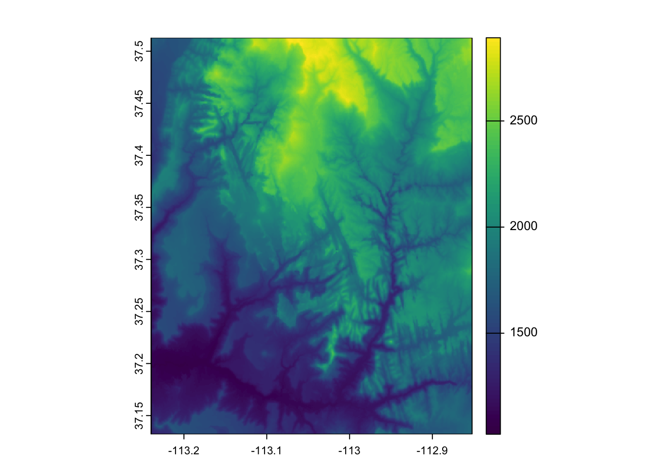
For the illustration of terra concepts, we will use datasets from the {spDataLarge} (Nowosad and Lovelace 2023). It consists of a few raster objects and one vector object covering an area of Zion National Park (Utah, USA). For example, srtm.tif is a digital elevation model of this area (SRMT stands for Shuttle Radar Topography Mission). Let’s create a SpatRaster object and get information about its class and content.

Code Collection 2.9 : Introduction to {terra} functions

SpatRaster object

R Code 2.32 : Create a SpatRaster object from “srtm.tif”

raster_filepath = base::system.file("raster/srtm.tif", package = "spDataLarge")
my_rast = terra::rast(raster_filepath)
base::class(my_rast)

#> [1] "SpatRaster"
#> attr(,"package")
#> [1] "terra"

my_rast

#> class       : SpatRaster 
#> dimensions  : 457, 465, 1  (nrow, ncol, nlyr)
#> resolution  : 0.0008333333, 0.0008333333  (x, y)
#> extent      : -113.2396, -112.8521, 37.13208, 37.51292  (xmin, xmax, ymin, ymax)
#> coord. ref. : lon/lat WGS 84 (EPSG:4326) 
#> source      : srtm.tif 
#> name        : srtm 
#> min value   : 1024 
#> max value   : 2892

my_rast2 <- terra::wrap(my_rast)
my_rast2

#> [1] "This is a PackedSpatRaster object. Use 'terra::unwrap()' to unpack it"

---

The name of the raster will print out the raster header (dimensions, resolution, extent, CRS) and some additional information (class, data source, and a summary of the raster values).

Watch out! 2.1: SpatRaster objects do not store raster values

Most SpatRaster objects do not store raster values, but rather a pointer to the file itself. This has a significant side-effect – they cannot be directly saved to .rds or .rda files or used in a different R session. Therefore I got

Error in .External(): ! NULL value passed as symbol address.

When I ran the code chunk in R Code 2.34 as terra::plot(my_rast) it worked, but I got the error whenever I rendered the whole document.

In these cases, there are two main possible solutions:

1. use of the terra::wrap() function that creates a special kind of temporary object that can be saved as an R object or used in cluster computing, or
2. save the object as a regular raster with terra::writeRaster() as I have done i R Code 2.37.

Using the values of SpatRaster in another session one needs to terra::unwrap() the object as I have done in R Code 2.34.

Raster header

R Code 2.33 : Reporting each component of the raster header with dedicated functions

base::dim(my_rast)          # returns the number of rows, columns and layers; 

#> [1] 457 465   1

terra::ncell(my_rast)       # returns the number of cells (pixels); 

#> [1] 212505

terra::res(my_rast)         # returns the spatial resolution; 

#> [1] 0.0008333333 0.0008333333

terra::ext(my_rast)         # return the spatial extent; and 

#> SpatExtent : -113.239583212784, -112.85208321281, 37.1320834298579, 37.5129167631658 (xmin, xmax, ymin, ymax)

terra::crs(my_rast)         # return the CRS  

#> [1] "GEOGCRS[\"WGS 84\",\n    ENSEMBLE[\"World Geodetic System 1984 ensemble\",\n        MEMBER[\"World Geodetic System 1984 (Transit)\"],\n        MEMBER[\"World Geodetic System 1984 (G730)\"],\n        MEMBER[\"World Geodetic System 1984 (G873)\"],\n        MEMBER[\"World Geodetic System 1984 (G1150)\"],\n        MEMBER[\"World Geodetic System 1984 (G1674)\"],\n        MEMBER[\"World Geodetic System 1984 (G1762)\"],\n        MEMBER[\"World Geodetic System 1984 (G2139)\"],\n        ELLIPSOID[\"WGS 84\",6378137,298.257223563,\n            LENGTHUNIT[\"metre\",1]],\n        ENSEMBLEACCURACY[2.0]],\n    PRIMEM[\"Greenwich\",0,\n        ANGLEUNIT[\"degree\",0.0174532925199433]],\n    CS[ellipsoidal,2],\n        AXIS[\"geodetic latitude (Lat)\",north,\n            ORDER[1],\n            ANGLEUNIT[\"degree\",0.0174532925199433]],\n        AXIS[\"geodetic longitude (Lon)\",east,\n            ORDER[2],\n            ANGLEUNIT[\"degree\",0.0174532925199433]],\n    USAGE[\n        SCOPE[\"Horizontal component of 3D system.\"],\n        AREA[\"World.\"],\n        BBOX[-90,-180,90,180]],\n    ID[\"EPSG\",4326]]"

terra::inMemory(my_rast)    # reports whether the raster data is stored in memory or on disk, and 

#> [1] FALSE

terra::sources(my_rast)     # specifies the file location

#> [1] "/Library/Frameworks/R.framework/Versions/4.4-x86_64/library/spDataLarge/raster/srtm.tif"

---

Dedicated functions report each component of the raster header (dimensions, resolution, extent, CRS) and some additional information (class, data source, summary of the raster values):

• base::dim() returns the number of rows, columns and layers;
• terra::ncell() returns the number of cells (pixels);
• terra::res() returns the spatial resolution;
• terra::ext() return the spatial extent; and
• terra::crs() return the CRS (raster reprojection is covered in (XXXSection7-8?)).
• terra::inMemory() reports whether the raster data is stored in memory or on disk, and
• terra::sources() specifies the file location.

The function terra::dim() didn’t work for me but it should be on of the “dedicated functions” of {terra}. I had to replace it with base::dim().

Remark 2.2. : {terra} package not essential for my use cases

As I am mostly interested to compare parameters for different countries it seems to me that vector data are the data type I have to go with.

Note 2.4: Overview of all {terra} functions

Typing help("terra-package") into the console you will get a list of all available {terra} function in the package help file. The same information you will get as an article in the package description on the web.

2.3.3 Basic map-making

Similar to the {sf} package, {terra} also provides plot() methods for its own classes.

R Code 2.34 : Basic map-making

terra::plot(terra::unwrap(my_rast2))

---

I have used here terra::unwrap(my_rast2) to prevent an error described in Warning 2.1.

There are several other approaches for plotting raster data in R that are outside the scope of this section, including:

• terra::plotRGB() function from the terra package to create a plot based on three layers in a SpatRaster object
• Packages such as {tmap} to create static and interactive maps of raster and vector objects (see (XXXChapter9?))
• Functions, for example rasterVis::levelplot() from the {rasterVis} package, to create facets, a common technique for visualizing change over time

2.3.4 Raster classes

The SpatRaster class represents rasters object of {terra}. The easiest way to create a raster object in R is to read-in a raster file from disk or from a server ((XXXSection8-3-2?)).

Code Collection 2.10 : Create a raster object

Reading file

R Code 2.35 : Create a raster object by reading a file from disk or server

raster_filepath = base::system.file("raster/srtm.tif", package = "spDataLarge")
single_rast = terra::rast(raster_filepath)

---

I had to change “single_raster_file” in the first line to raster_filepath. Should I create a pull request (PR) to patch this mistake?

The {terra} package supports numerous drivers with the help of the GDAL library. With terra::gdal(drivers = TRUE) you will get all the 200 different drivers that are available to date (2025-02-02) or (even better) use the up-to-date GDAL web documented list of drivers. GDAL is the software library that {terra} builds on to read and write spatial data and for some raster data processing.

These classes hold a C++ pointer to the data “reference class” and that creates some limitations. They cannot be recovered from a saved R session either or directly passed to nodes on a computer cluster. Generally, you should use terra::writeRaster() to save SpatRaster objects to disk (and pass a filename or cell values of cluster nodes). See for example R Code 2.37. Or use terra::wrap() as I have done in R Code 2.32.

From scratch

R Code 2.36 : Create raster object from scratch

new_raster = terra::rast(nrows = 6, ncols = 6, 
                  xmin = -1.5, xmax = 1.5, ymin = -1.5, ymax = 1.5,
                  vals = 1:36)
new_raster

#> class       : SpatRaster 
#> dimensions  : 6, 6, 1  (nrow, ncol, nlyr)
#> resolution  : 0.5, 0.5  (x, y)
#> extent      : -1.5, 1.5, -1.5, 1.5  (xmin, xmax, ymin, ymax)
#> coord. ref. : lon/lat WGS 84 
#> source(s)   : memory
#> name        : lyr.1 
#> min value   :     1 
#> max value   :    36

---

Rasters can also be created from scratch, illustrated in the above code chunk. The resulting raster consists of 36 cells (6 columns and 6 rows specified by nrows and ncols) centered around the Prime Meridian and the Equator (see xmin, xmax, ymin and ymax parameters). Values (vals) are assigned to each cell: 1 to cell 1, 2 to cell 2, and so on. Remember: terra::rast() fills cells row-wise (unlike base::matrix()) starting at the upper left corner, meaning the top row contains the values 1 to 6, the second 7 to 12, etc. Raster objects can also created from another object (see: Create a SpatRaster).

Given the number of rows and columns as well as the extent (xmin, xmax, ymin, ymax), the resolution has to be 0.5. The unit of the resolution is that of the underlying CRS. Here, it is degrees, because the default CRS of raster objects is WGS84. However, one can specify any other CRS with the crs argument.

The SpatRaster class also handles multiple layers, which typically correspond to a single multi-spectral satellite file or a time-series of rasters.

Code Collection 2.11 : Handling multiple raster layers

Create multi raster

R Code 2.37 : Creating raster with multiple layers

multi_raster_file = base::system.file("raster/landsat.tif", package = "spDataLarge")
multi_rast = terra::rast(multi_raster_file)
multi_rast

#> class       : SpatRaster 
#> dimensions  : 1428, 1128, 4  (nrow, ncol, nlyr)
#> resolution  : 30, 30  (x, y)
#> extent      : 301905, 335745, 4111245, 4154085  (xmin, xmax, ymin, ymax)
#> coord. ref. : WGS 84 / UTM zone 12N (EPSG:32612) 
#> source      : landsat.tif 
#> names       : landsat_1, landsat_2, landsat_3, landsat_4 
#> min values  :      7550,      6404,      5678,      5252 
#> max values  :     19071,     22051,     25780,     31961

pb_create_folder("data")
pb_create_folder("data/Chapter2")

terra::writeRaster(
  multi_rast,
  "data/Chapter2/landsat.tif",
  overwrite = TRUE,
  datatype = "FLT4S"
  ) 

Raster layers

R Code 2.38 : Get number of raster layers

multi_rast <- terra::rast("data/Chapter2/landsat.tif")


terra::nlyr(multi_rast)

#> [1] 4

Select & combine layers

R Code 2.39 : Select (subset) raster layers

multi_rast <- terra::rast("data/Chapter2/landsat.tif")

multi_rast3 = terra::subset(multi_rast, 3)
multi_rast4 = terra::subset(multi_rast, "landsat_4")

multi_rast34 = base::c(multi_rast3, multi_rast4)

As SpatRaster objects do not save the data but only a pointer I had to look ahead to (XXXSection8-4-2?). and save the SpatRaster object with terra::writeRaster() to the disk. Then I had always to load the saved .tif object and restore is as SpatRaster object with terra::rast(). I do not know yet if this cumbersome method (always creating ) is correct or if there is a simpler posssibility. (See for instance the discussion on GitHub)

2.4 Coordinate Reference Systems

The coordinate reference systems (CRSs) defines how the spatial elements of the data relate to the surface of the Earth (or other bodies). CRSs are either geographic or projected.

2.4.1 Geographic coordinate reference systems

Geographic CRSs identify any location on the Earth’s surface using two values — longitude and latitude. Longitude is location in the East-West direction in angular distance from the Prime Meridian plane. Latitude is angular distance North or South of the equatorial plane. Distances in geographic CRSs are therefore not measured in meters. This has important consequences, as demonstrated in (XXXChapter7?).

The surface of the Earth in geographic CRSs is represented by a spherical or ellipsoidal surface. Spherical models assume that the Earth is a perfect sphere of a given radius – they have the advantage of simplicity but, at the same time, they are inaccurate as the Earth is not exactly a sphere. Ellipsoidal models are slightly more accurate, and are defined by two parameters: the equatorial radius and the polar radius. These are suitable because the Earth is compressed: the equatorial radius is around 11.5 km longer than the polar radius (Maling 1992).

The datum contains information on what ellipsoid to use and the precise relationship between the coordinates and location on the Earth’s surface. There are two types of datum — geocentric (such as WGS84) and local (such as NAD83).

You can see examples of these two types of datums in Figure 2.15. Black lines represent a geocentric datum, whose center is located in the Earth’s center of gravity and is not optimized for a specific location. In a local datum, shown as a purple dashed line, the ellipsoidal surface is shifted to align with the surface at a particular location. These allow local variations in Earth’s surface, for example due to large mountain ranges, to be accounted for in a local CRS. This can be seen in Figure 2.15, where the local datum is fitted to the area of Philippines, but is misaligned with most of the rest of the planet’s surface. Both datums in Figure 2.15 are put on top of a geoid — a model of global mean sea level.

Figure 2.15: Geocentric and local geodetic datums shown on top of a geoid (in false color and the vertical exaggeration by 10,000 scale factor). Image of the geoid is adapted from the work of Ince et al. (Ince et al. 2019; International Centre for Global Earth Models 2025)

2.4.2 Projected coordinate reference systems

All projected CRSs are based on a geographic CRS, described in the previous section, and rely on map projections to convert the three-dimensional surface of the Earth into Easting and Northing (x and y) values in a projected CRS. Projected CRSs are based on Cartesian coordinates on an implicitly flat surface (Figure 2.17, right panel). They have an origin, x and y axes, and a linear unit of measurement such as meters.

This transition cannot be done without adding some deformations. Therefore, some properties of the Earth’s surface are distorted in this process, such as area, direction, distance, and shape. A projected coordinate reference system can preserve only one or two of those properties. Projections are often named based on a property they preserve: For instance

• equal-area preserves area,
• azimuthal preserve direction,
• equidistant preserve distance, and
• conformal preserve local shape.

There are three main groups of projection types: conic, cylindrical, and planar (azimuthal).

• In a conic projection, the Earth’s surface is projected onto a cone along a single line of tangency or two lines of tangency. Distortions are minimized along the tangency lines and rise with the distance from those lines in this projection. Therefore, it is the best suited for maps of mid-latitude areas.
• A cylindrical projection maps the surface onto a cylinder. This projection could also be created by touching the Earth’s surface along a single line of tangency or two lines of tangency. Cylindrical projections are used most often when mapping the entire world.
• A planar projection projects data onto a flat surface touching the globe at a point or along a line of tangency. It is typically used in mapping polar regions.

Resource 2.2 : Projections supported by the PROJ library

• sf::sf_proj_info(type = "proj") gives a list of the current 178 available projections supported by the PROJ library.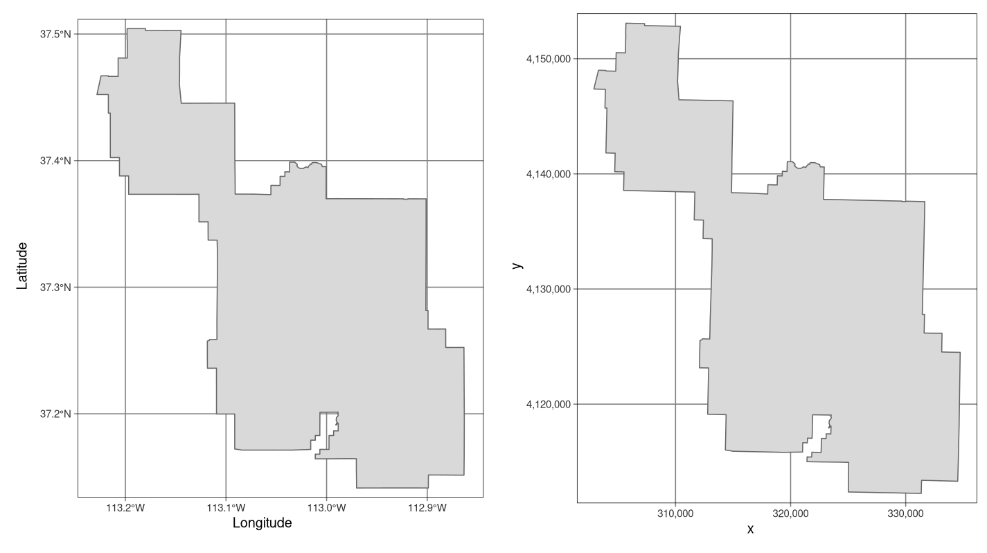
• See also details for each projection type that map the spherical 3D space to a flat 2D space at the PROJ website.
• A quick summary of different projections, their types, properties, and suitability can be explored with the Map Projection Explorer at www.geo-projections.com.

---

Figure 2.16: Examples of geographic (WGS84; left) and projected (NAD83 / UTM zone 12N; right) coordinate systems for a vector data type.

---

Summary of CRS section

We will expand on CRSs and explain how to project from one CRS to another in (XXXChapter7?). For now, it is sufficient to know:

• Coordinate systems are a key component of geographic objects
• Which CRS your data is in, and whether it is in geographic (lon/lat) or projected (typically meters), is important and has consequences for how R handles spatial and geometry operations
• CRSs of {sf} objects can be queried with the function sf::st_crs() and CRSs of {terra} objects can be queried with the function terra::crs().

2.5 Units

An important feature of CRSs is that they contain information about spatial units. It is good cartographic practice to add a scale bar or some other distance indicator onto maps to demonstrate the relationship between distances on the page or screen and distances on the ground. Likewise, it is important to formally specify the units in which the geometry data or cells are measured to provide context, and to ensure that subsequent calculations are done in the correct context.

2.5.1 Units in sf

A novel feature of geometry data in sf objects is that they have native support for units. This means that distance, area and other geometric calculations in {sf} return values that come with a units attribute, defined by the units package (Pebesma, Mailund, and Hiebert 2016). (See Package Profile in Section A.6.)

Code Collection 2.12 : Calculating an area as a {sf} units example

Area calculation

R Code 2.40 : Calculation the Area of Luxembourg

utils::data("world", package = "spData")

(
  luxembourg <- world |> 
    dplyr::filter(name_long == "Luxembourg") |> 
    sf::st_area() # requires {s2} in recent versions of {sf}
)

#> 2408817306 [m^2]

base::attributes(luxembourg)

#> $units
#> $numerator
#> [1] "m" "m"
#> 
#> $denominator
#> character(0)
#> 
#> attr(,"class")
#> [1] "symbolic_units"
#> 
#> $class
#> [1] "units"

Unit conversion

R Code 2.41 : Translate m^2 into km^2

luxembourg / 1000000 # wrong

#> 2408.817 [m^2]

(
  luxembourg_km2 <- units::set_units(luxembourg, km^2) # correct
) 

#> 2408.817 [km^2]

base::attributes(luxembourg_km2)

#> $units
#> $numerator
#> [1] "km" "km"
#> 
#> $denominator
#> character(0)
#> 
#> attr(,"class")
#> [1] "symbolic_units"
#> 
#> $class
#> [1] "units"

2.5.2 Units in terra

Units are of equal importance in the case of raster data. However, so far {sf} is the only spatial package that supports units, meaning that people working on raster data should approach changes in the units of analysis (for example, converting pixel widths from imperial to decimal units) with care. The my_rast object in R Code 2.32 uses a WGS84 projection with decimal degrees as units. Consequently, its resolution is also given in decimal degrees, but you have to know it, since the terra::res() function simply returns a numeric vector. And if we used the Universal Transverse Mercator (UTM) projection, the units would change and we would have to know that the units are now in meter.

R Code 2.42 : Units in {terra}

terra::res(terra::unwrap(my_rast2)) # units in decimal degress

#> [1] 0.0008333333 0.0008333333

repr = terra::project(terra::unwrap(my_rast2), "EPSG:26912") # UTM projection
terra::res(repr) # units in meter

#> [1] 83.53328 83.53328

2.6 Exercises

References

Cooley, David. 2024. “Sfheaders: Converts Between r Objects and Simple Feature Objects.” https://CRAN.R-project.org/package=sfheaders.

Evenden, Gerald I., Even Rouault, Frank Warmerdam, Kristian Evers, Thomas Knudsen, Howard Butler, Mike W. Taves, et al. 2024. PROJ Coordinate Transformation Software Library. Zenodo. https://doi.org/10.5281/ZENODO.5884394.

GEOS contributors. 2024. “GEOS Computational Geometry Library.” https://doi.org/10.5281/zenodo.11396894.

Ince, E. Sinem, Franz Barthelmes, Sven Reißland, Kirsten Elger, Christoph Förste, Frank Flechtner, and Harald Schuh. 2019. “ICGEM 15 Years of Successful Collection and Distribution of Global Gravitational Models, Associated Services, and Future Plans.” Earth System Science Data 11 (2): 647–74. https://doi.org/10.5194/essd-11-647-2019.

International Centre for Global Earth Models. 2025. “Visualization of Gravity Field Models and Their Differences.” https://icgem.gfz-potsdam.de/vis3d/longtime.

Maling, D. H. 1992. Coordinate Systems and Map Projections. Subsequent Edition. Oxford ; New York: Butterworth-Heinemann Ltd.

Pebesma, Edzer, and Roger Bivand. 2023. Spatial Data Science: With Applications in R. 1st ed. Boca Raton London New York: CRC Press.

Pebesma, Edzer, Thomas Mailund, and James Hiebert. 2016. “Measurement Units in r” 8. https://doi.org/10.32614/RJ-2016-061.

Rouault, Even, Frank Warmerdam, Kurt Schwehr, Andrey Kiselev, Howard Butler, Mateusz Łoskot, Tamas Szekeres, et al. 2025. GDAL. Zenodo. https://doi.org/10.5281/ZENODO.5884351.

S2 Geometry Library Contributors. 2025. S2 Geometry. Google. http://s2geometry.io/.

Sadler, Jesse. 2018. “An Exploration of Simple Features for R.” https://www.jessesadler.com/post/simple-feature-objects/.

---

1. Thus to store many values for a single location we need to have many raster layers.