Chapter 2 Introduction
吴恩达机器学习 - 网易云课堂 吴恩达机器学习 中英字幕B站版本
Great music to listen while studying: Figlia del cielo III
[[吴恩达机器学习课程及多版本笔记纲要]]
You can label chapter and section titles using {#label} after them, e.g., we can reference Chapter 2. If you do not manually label them, there will be automatic labels anyway, e.g., Chapter 4.
Figures and tables with captions will be placed in figure and table environments, respectively.
par(mar = c(4, 4, .1, .1))
plot(pressure, type = 'b', pch = 19)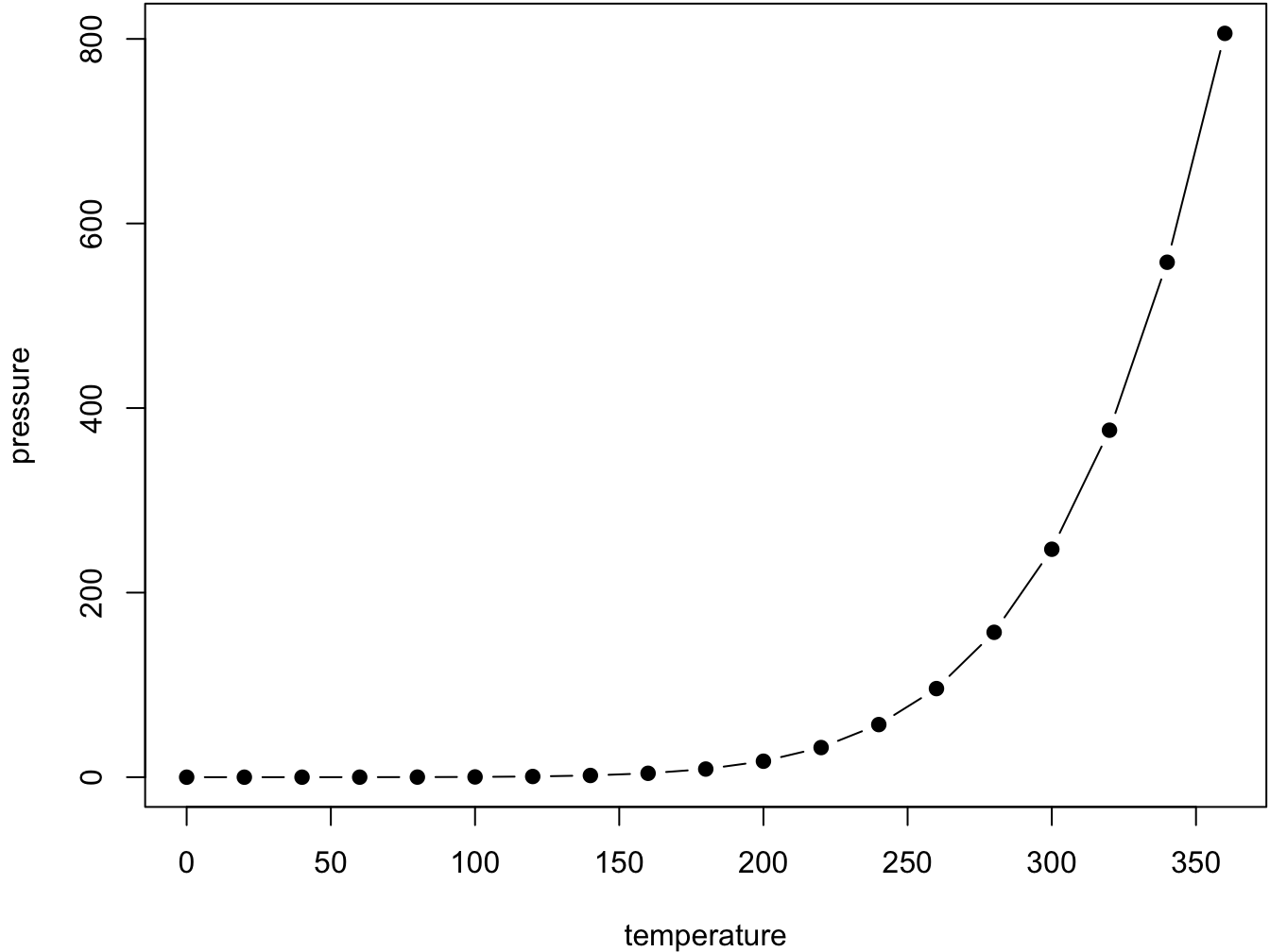
Figure 2.1: Here is a nice figure!
Reference a figure by its code chunk label with the fig: prefix, e.g., see Figure 2.1. Similarly, you can reference tables generated from knitr::kable(), e.g., see Table 2.1.
knitr::kable(
  head(iris, 20), caption = 'Here is a nice table!',
  booktabs = TRUE
)| Sepal.Length | Sepal.Width | Petal.Length | Petal.Width | Species |
|---|---|---|---|---|
| 5.1 | 3.5 | 1.4 | 0.2 | setosa |
| 4.9 | 3.0 | 1.4 | 0.2 | setosa |
| 4.7 | 3.2 | 1.3 | 0.2 | setosa |
| 4.6 | 3.1 | 1.5 | 0.2 | setosa |
| 5.0 | 3.6 | 1.4 | 0.2 | setosa |
| 5.4 | 3.9 | 1.7 | 0.4 | setosa |
| 4.6 | 3.4 | 1.4 | 0.3 | setosa |
| 5.0 | 3.4 | 1.5 | 0.2 | setosa |
| 4.4 | 2.9 | 1.4 | 0.2 | setosa |
| 4.9 | 3.1 | 1.5 | 0.1 | setosa |
| 5.4 | 3.7 | 1.5 | 0.2 | setosa |
| 4.8 | 3.4 | 1.6 | 0.2 | setosa |
| 4.8 | 3.0 | 1.4 | 0.1 | setosa |
| 4.3 | 3.0 | 1.1 | 0.1 | setosa |
| 5.8 | 4.0 | 1.2 | 0.2 | setosa |
| 5.7 | 4.4 | 1.5 | 0.4 | setosa |
| 5.4 | 3.9 | 1.3 | 0.4 | setosa |
| 5.1 | 3.5 | 1.4 | 0.3 | setosa |
| 5.7 | 3.8 | 1.7 | 0.3 | setosa |
| 5.1 | 3.8 | 1.5 | 0.3 | setosa |
You can write citations, too. For example, we are using the bookdown package (Xie 2018) in this sample book, which was built on top of R Markdown and knitr (Xie 2015).
References
Xie, Yihui. 2018. Bookdown: Authoring Books and Technical Documents with R Markdown. https://CRAN.R-project.org/package=bookdown.
Xie, Yihui. 2015. Dynamic Documents with R and Knitr. 2nd ed. Boca Raton, Florida: Chapman; Hall/CRC. http://yihui.name/knitr/.