Chapter 8 Modeling
8.1 Simple Linear Regression
Predicting Winning Percentage
For this section we will be using the Teams table.
team_pred <- Teams %>%
  filter(yearID >= 2012, yearID < 2020)
Say we want to predict winning percentage using a team’s run differential. To do this we need to create two new variables: run differential (RD) and winning percentage (WPCT). Run differential is calculated with runs scored (R) and runs allowed (RA). Calculating winning percentage requires the amount of wins and losses.
team_pred <- team_pred %>%
  mutate(RD = R - RA,
         WPCT = W / (W + L))
Now it’s time to build the model. The lm() function is used to fit linear models. It requires a formula, following the format: response ~ predictor(s). A response variable is the variable we are trying to predict. Predictor variables are used to make predictions. In this example, we will predict a team’s winning percentage (response) using its run differential (predictor).
model1 <- lm(WPCT ~ RD, data = team_pred)
model1
##
## Call:
## lm(formula = WPCT ~ RD, data = team_pred)
##
## Coefficients:
## (Intercept) RD
## 0.4999830 0.0006089The general equation of a simple linear regression line is: \(\hat{y} = b_0 + b_1 x\). The symbols have the following meaning:
- \(\hat{y}\) = predicted value of the response variable
- \(b_0\) = estimated y-intercept for the line
- \(b_1\) = estimated slope for the line
- x = predictor value to plug in
This output provides us with an equation we can use to predict a team’s winning percentage based on their run differential:
\[\text{Predicted Win Pct} = 0.500 + 0.00061 * \text{Run Diff}\]
The estimated y-intercept for this model is 0.500. This means that we would predict a winning percentage of 0.500 for a team with a run differential of 0. In other words, teams who give up and score the same number of runs are predicted to be average. This makes a lot of sense for this example, but we will see later that y-intercept interpretations aren’t always applicable like this.
The slope for this model is 0.0006267. There are 162 games in the MLB regular season. If we multiple the slope by 162 we get 0.1015, which equates to 1/10th of a win. For each additional difference the predicted wins goes up by 0.0006. This works out to about 0.1 wins.
The estimate slope for our line is 0.00061. This tells us that our predicted winning percentage increases by 0.00061 for each additional run a team scores (or each fewer run they allow). Over a 162 game season, a change in winning percentage of 0.00061 is equivalent to around \(162 * 0.00061 = 0.1\) wins. In other words, an increase of around 10 runs scored (or prevented) is associated with around 1 more win in a season.
The summary() function can give us some additional information about our linear regression model.
summary(model1)##
## Call:
## lm(formula = WPCT ~ RD, data = team_pred)
##
## Residuals:
## Min 1Q Median 3Q Max
## -0.060481 -0.016448 0.000136 0.014840 0.081565
##
## Coefficients:
## Estimate Std. Error t value Pr(>|t|)
## (Intercept) 5.000e-01 1.630e-03 306.74 <2e-16 ***
## RD 6.089e-04 1.414e-05 43.05 <2e-16 ***
## ---
## Signif. codes: 0 '***' 0.001 '**' 0.01 '*' 0.05 '.' 0.1 ' ' 1
##
## Residual standard error: 0.02525 on 238 degrees of freedom
## Multiple R-squared: 0.8862, Adjusted R-squared: 0.8857
## F-statistic: 1854 on 1 and 238 DF, p-value: < 2.2e-16Another important thing to look at is the p-value. A p-value tells us how likely certain results would be to occur if “nothing was going on”. We often compare a p-value to a pre-chosen significance level, alpha, to decide if our results would be unusual in a world where our variables weren’t related to one another. The most frequently used significance level is alpha = 0.5. Our model’s p-value is less than 2.2e-16, or 0.00000000000000022, which is much smaller than alpha. This suggests that run differential is helpful in predicting winning percentage because results like this are incredibly unlikely to occur if the two variables are not related.
R-squared values are used to describe how well the model fits the data. In this model, the R-squared value is 0.8862. This is saying that around 88.6% of variability in team winning percentage is explained by run differential.
This should not be the exclusive method to assess model fit, but it helps give us a good idea.
To visualize this data we can make a scatter plot and fit a line using geom_smooth(). If no method is specified, R will automatically fit the model it thinks is best. Since we fit a linear model above, the method should be “lm”.
team_pred %>%
  ggplot(aes(x = RD, y = WPCT)) +
  geom_point(alpha = 0.5) +
  geom_smooth(method = "lm") +
  theme_bw() +
theme(text = element_text(family = "serif")) 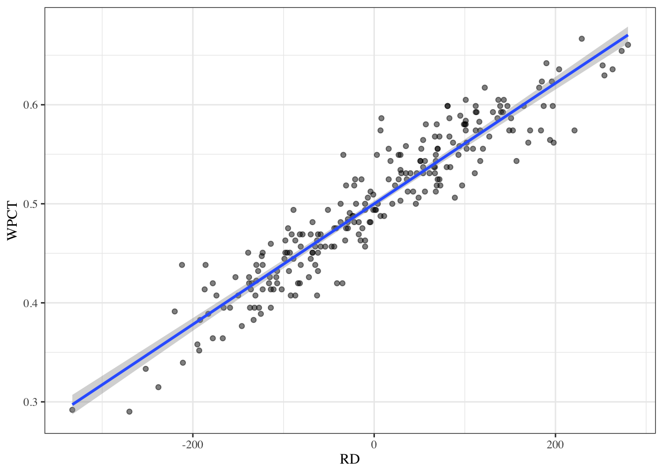
8.2 Multiple Linear Regression
Linear Weights
We are going to predict runs using singles, doubles, triples, homeruns, walks, hit-by-pitches, strikeouts, non-strikeouts, stolen bases,caught stealing, and sacrifice flies.
First, we need to create a variable for singles (‘X1B’) and a variable for non-strikeouts (‘nonSO’).
team_pred <- team_pred %>%
  mutate(X1B = H - X2B - X3B - HR,
         nonSO = AB - H - SO)
model2 <- lm(R ~ X1B + X2B + X3B + HR + BB + HBP + SO + nonSO + SB + CS + SF,
data = team_pred)
summary(model2)##
## Call:
## lm(formula = R ~ X1B + X2B + X3B + HR + BB + HBP + SO + nonSO +
## SB + CS + SF, data = team_pred)
##
## Residuals:
## Min 1Q Median 3Q Max
## -47.801 -14.369 0.892 13.045 69.662
##
## Coefficients:
## Estimate Std. Error t value Pr(>|t|)
## (Intercept) -81.29410 148.23774 -0.548 0.58395
## X1B 0.39790 0.03233 12.308 < 2e-16 ***
## X2B 0.85072 0.06261 13.588 < 2e-16 ***
## X3B 1.03915 0.17326 5.998 7.78e-09 ***
## HR 1.46743 0.04932 29.755 < 2e-16 ***
## BB 0.27182 0.02782 9.771 < 2e-16 ***
## HBP 0.42774 0.10060 4.252 3.09e-05 ***
## SO -0.07632 0.03220 -2.370 0.01863 *
## nonSO -0.06348 0.03324 -1.910 0.05743 .
## SB 0.19423 0.06119 3.174 0.00171 **
## CS -0.48735 0.21521 -2.265 0.02448 *
## SF 0.54252 0.20891 2.597 0.01002 *
## ---
## Signif. codes: 0 '***' 0.001 '**' 0.01 '*' 0.05 '.' 0.1 ' ' 1
##
## Residual standard error: 21.41 on 228 degrees of freedom
## Multiple R-squared: 0.9264, Adjusted R-squared: 0.9228
## F-statistic: 260.7 on 11 and 228 DF, p-value: < 2.2e-16Most of the p-values from this model have stars next to them. ** is significant at alpha = 0.001. *** is significant at alpha = 0.0001. The intercept’s p-value is the only one without stars. A p-value of 0.205166 suggests that we may not need the the intercept. This makes sense since a team that does none of these things (the predictor variables) would score 0 runs.
Now let’s try fitting a model with no intercept. We can accomplish this by putting “- 1” at the of the model equation.
model2 <- lm(R ~ X1B + X2B + X3B + HR + BB + HBP + SO + nonSO + SB + CS + SF - 1,
             data = team_pred)
summary(model2)
##
## Call:
## lm(formula = R ~ X1B + X2B + X3B + HR + BB + HBP + SO + nonSO +
## SB + CS + SF - 1, data = team_pred)
##
## Residuals:
## Min 1Q Median 3Q Max
## -48.007 -13.854 0.806 13.124 68.714
##
## Coefficients:
## Estimate Std. Error t value Pr(>|t|)
## X1B 0.39069 0.02949 13.250 < 2e-16 ***
## X2B 0.85139 0.06250 13.622 < 2e-16 ***
## X3B 1.03696 0.17295 5.996 7.82e-09 ***
## HR 1.46023 0.04746 30.764 < 2e-16 ***
## BB 0.26889 0.02726 9.864 < 2e-16 ***
## HBP 0.42671 0.10043 4.249 3.13e-05 ***
## SO -0.09296 0.01073 -8.664 8.36e-16 ***
## nonSO -0.08080 0.01037 -7.793 2.28e-13 ***
## SB 0.19452 0.06109 3.184 0.00165 **
## CS -0.51889 0.20707 -2.506 0.01291 *
## SF 0.53251 0.20779 2.563 0.01103 *
## ---
## Signif. codes: 0 '***' 0.001 '**' 0.01 '*' 0.05 '.' 0.1 ' ' 1
##
## Residual standard error: 21.38 on 229 degrees of freedom
## Multiple R-squared: 0.9992, Adjusted R-squared: 0.9991
## F-statistic: 2.453e+04 on 11 and 229 DF, p-value: < 2.2e-16This model’s p-value is 2.2e-16, which is incredibly small. The R-squared value is 0.9992, meaning that 99.9% of variability in runs is explained by these 10 variables.
Here is a table of the of each MLR variable and their slope:
kable(model2$coefficients, col.names = "Coefficient") %>%
kable_styling("striped", full_width = FALSE)| Coefficient | |
|---|---|
| X1B | 0.3906859 |
| X2B | 0.8513918 |
| X3B | 1.0369631 |
| HR | 1.4602320 |
| BB | 0.2688928 |
| HBP | 0.4267069 |
| SO | -0.0929639 |
| nonSO | -0.0807959 |
| SB | 0.1945239 |
| CS | -0.5188885 |
| SF | 0.5325096 |
The coefficient for stolen bases is 0.1945. This means that a team will score 0.1945 runs for every base they steal, given that all other variables remain constant. A coefficient of -0.5191 for caught stealing is saying that the number of runs will decrease by -0.5191 for every time the team is caught stealing.
To see how good this model is we will plot the predicted runs against the actual runs. The line represents a perfect model.
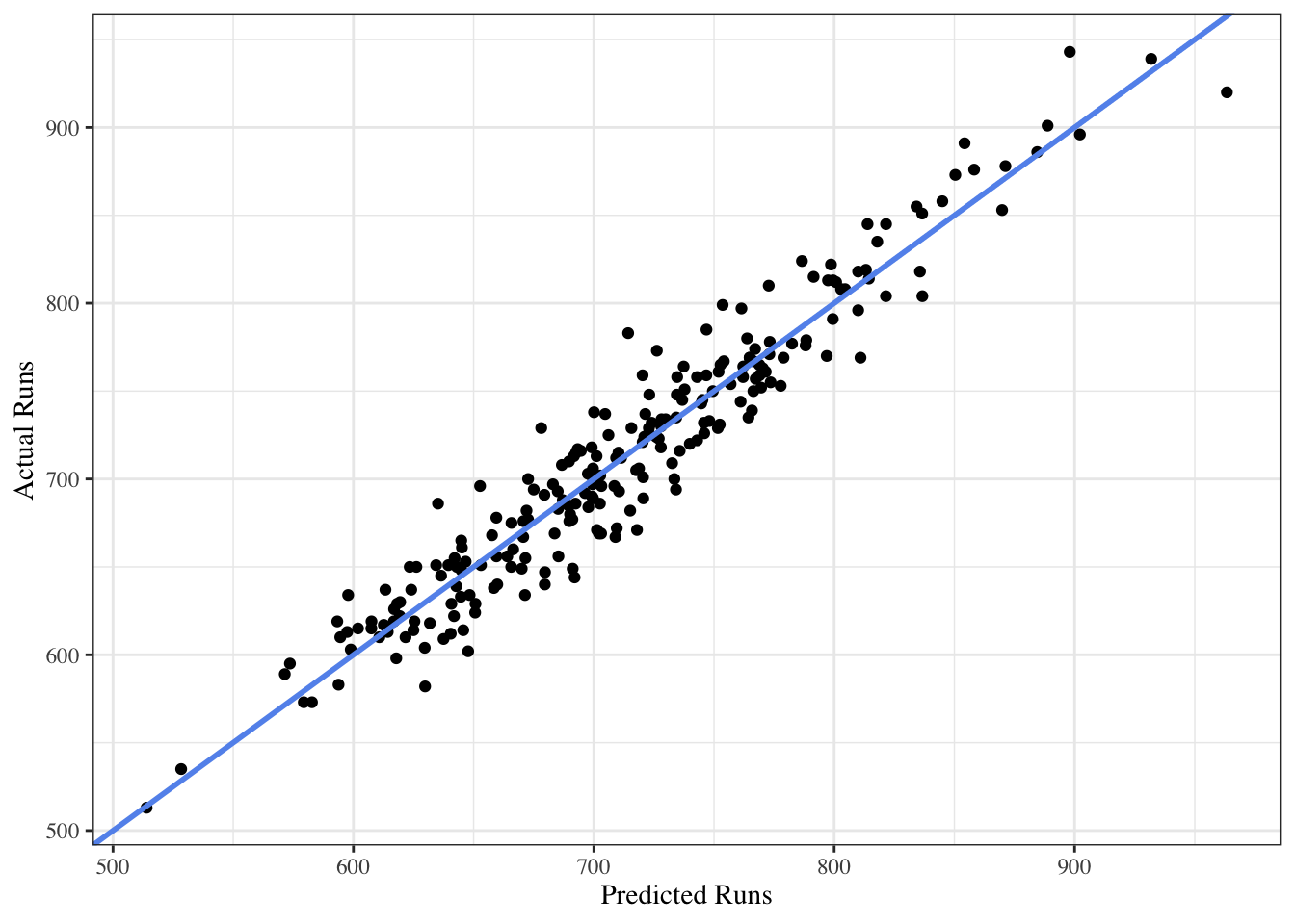
The points stay close to the line, which indicates that the model fits the data very well. This supports the same conclusion as the R-squared value.
8.3 Logistic Regression
Similar to linear regression, logistic regression uses one or more variables to predict another variable. However, the response variables for logistic regression are binary, meaning there are only two options. Common examples include options like Yes/No, 1/0 or True/False.
Let’s put this into application.
8.3.1 Predicting the Odds of > 0 WAR by Overall Draft Pick Number
For this section, we will be using the all_draft dataset that was first created in the Web-Scraping Section of this book.
all_draft <- read.csv("https://raw.githubusercontent.com/vank-stats/Baseball-Analytics-Guide/main/data/draft_data.csv")For this example, we will be predicting the likelihood that a first round pick achieves more than 0 career WAR (binary response variable). We will use the pick number to help us with our prediction.
The all_draft data gives the career WAR of players, but we must create a new variable to determine whether a first round pick accrued more than 0 WAR in their career. This will give us the binary variable we need for our logistic regression response variable.
In this example, the variable Positive is coded as:
- 0: the player did not make the majors (WAR is NA in the data)
- 0: the player made the majors but had less than or equal to one career WAR
- 1: the player had more than zero career WAR (which is anything else)
all_draft <- mutate(all_draft,
                    Positive = case_when(is.na(WAR) ~ 0,
                                         WAR <= 0 ~ 0,
                                         TRUE ~ 1))
Unlike linear regression, where we are predicting a quantitative response variable, logistic regressions are used to predict the log odds of a binary response. In notation, that looks like:
\[\widehat{log\Big(\frac{p}{1-p}\Big)} = b_0 + b_1x\] In the equation above, the response variable is the log odds of earning more than 0 WAR in the majors. The “^” symbol above the left hand side of the equation means that we are predicting that value. Therefore, we are predicting the log odds in the above equation.
Now we can interpret each variable:
- \(b_0\) = estimated y-intercept
- \(b_1\) = estimated slope
- \(x\) = predictor value being plugged in
- \(p\) = probability of “success” for a specified value of x
- \(\frac{p_i}{1-p_i}\) = odds of “success” (probability of success divided by one minus probability of success)
For logistic regression, we will use a function called glm(). This function is designed to fit logistic regression models, while the lm() function is designed to fit linear regression models. Both functions work in similar ways using the response ~ explanatory format. To run a logistic regression model, we will set the family argument equal to binomial in the glm() function.
war_glm <- glm(Positive ~ OvPck,
               family = binomial,
               data = all_draft)
war_glm
##
## Call: glm(formula = Positive ~ OvPck, family = binomial, data = all_draft)
##
## Coefficients:
## (Intercept) OvPck
## 1.15011 -0.03988
##
## Degrees of Freedom: 500 Total (i.e. Null); 499 Residual
## Null Deviance: 693.3
## Residual Deviance: 649.3 AIC: 653.3For this model, success is a response value of 1 (aka a player accruing more than 0 career WAR)
Using the values from our logistic regression output, the equation becomes:
\[\widehat{log\Big(\frac{p}{1-p}\Big)} = 1.15011 - 0.03988 * \text{Draft Spot}\] The y-intercept and slope can be interpreted similarly to how they were done in simple linear regression (but for a predicted log odds of our response variable).
The estimated y-intercept for the model is 1.15011. This means we predict a log odds of more than one career WAR of 1.15011 when a player is drafted with the number 0 overall pick.
The estimated slope for the model is -0.03988. This tells us that the predicted log odds of more than one career WAR decreases by roughly 0.04 for each additional pick spot (e.g. moving from the 1st to the 2nd overall pick or from the 30th to the 31st overall pick).
As you can see, these interpretations have almost no practical meaning and are difficult to interpret since few people have a good intuition about changes in log odds. However, we can convert the equation to predicting odds instead of log odds by taking e to the power of both sides of the equation.
This leads to a new formula:
\[\widehat{\frac{p}{1-p}} = e^{1.15011 - 0.03988x}\] Ultimately, we want to find the probability that a player generates more than than one career WAR which requires us to isolate \(\widehat p\) in our equation. This can be done using algebra, which leads to a new formula for the predicted probability of more than one career WAR:
\[\widehat{p} = \frac{e^{{1.15011 - 0.03988x}}}{1 + e^{1.15011 - 0.03988x}}\] While this formula looks a little confusing, it will calculate exactly what we want. Now, by plugging in an overall pick number, we will get the predicted probability that the player will generate more than zero WAR.
For example, lets predict the probability that a number 1 overall pick will generate more than zero career WAR. To do this, we just need to plug 1 into our predicted probability formula for x. This will look like:
\[\widehat{p} = \frac{e^{{1.15011 - 0.03988(1)}}}{1 + e^{1.15011 - 0.03988(1)}} = 0.752\]
We can also use the predict() function to calculate predicted probabilities. Here is some code that will have R calculate this for us:
predict(war_glm, newdata= data.frame(OvPck = 1), type = "response")## 1
## 0.7521718(Note: The slight differences between the two predictions are due to rounding. In general, the predict() function will give a more accurate result as no rounding is performed in it.)
Instead of predicting individual values, we may want to visualize how the predictions change across the first round. The code below will add the predicted
odds as a variable in the data (using predict()). We can then calculate the predicted probabilities.
all_draft <- all_draft %>%
  mutate(prediction_log = predict(war_glm, all_draft),
         prediction = exp(prediction_log) / (1 + exp(prediction_log)))
The graph below plots the pick number on the x-axis and our predicted probability of more than one WAR on the y-axis. We can see that the top picks have around a 60 - 65% chance of accumulating at least zero WAR while that probability drops to around 50% at the 20th overall pick and around 25% at the 50th overall pick.
ggplot(all_draft, aes(x = OvPck, y = prediction)) +
  geom_line(linewidth = 1) +
  theme_bw() +
  lims(y = c(0, 1)) +
  labs(title = "Chances a First Round Draft Pick Achieves Positive WAR",
       caption = "Data collected from Baseball Reference (2004-2013)",
       x = "Overall Pick Number",
       y = "Predicted Probability")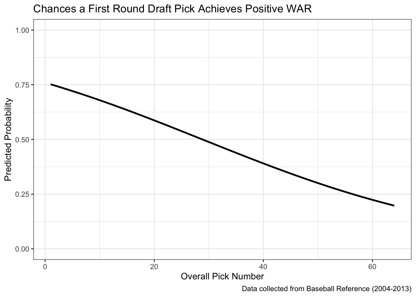
8.4 Logistic Regression (Multiple Explanatory Variables)
In order to finalize our dataset, we can create two new variables to help with our analysis: Position, and Type.
The variable Position indicates whether the player was a pitcher or hitter when they were drafted.
The variable Type shows where a player was drafted out of (4-Year College, High school, Junior College, Other). We are going to look at any differences between where players were drafted from next.
Additionally, we must add code that creates a reference value for the variable Type. When a model that contains categorical variables is created, one of the categories becomes the reference value that each of the other categories are compared to. Because there are very few observations in the categories, “JC” and ” “, we must be careful when choosing a reference variable. Since”4Yr” has the most observations, it becomes the most logical variable to become the reference value.
all_draft <- mutate(all_draft,
                      Position = ifelse(str_detect(Pos, "HP"),
                                        "pitcher",
                                        "hitter"),
                      Type = factor(Type, levels = c("4Yr", "HS", "JC", "")))
Using a similar approach to our previous example, lets fit a logistic regression model with multiple explanatory variables.
multiple_glm <- glm(Positive ~ OvPck + Position + Type,
               family = binomial,
               data = all_draft)
summary(multiple_glm)
##
## Call:
## glm(formula = Positive ~ OvPck + Position + Type, family = binomial,
## data = all_draft)
##
## Deviance Residuals:
## Min 1Q Median 3Q Max
## -1.7989 -1.1169 0.6894 1.0362 1.7275
##
## Coefficients:
## Estimate Std. Error z value Pr(>|z|)
## (Intercept) 1.235237 0.234824 5.260 1.44e-07 ***
## OvPck -0.040486 0.006425 -6.302 2.94e-10 ***
## Positionpitcher 0.242663 0.191817 1.265 0.2058
## TypeHS -0.448104 0.192924 -2.323 0.0202 *
## TypeJC 0.241506 0.679432 0.355 0.7223
## Type 0.924679 1.238653 0.747 0.4554
## ---
## Signif. codes: 0 '***' 0.001 '**' 0.01 '*' 0.05 '.' 0.1 ' ' 1
##
## (Dispersion parameter for binomial family taken to be 1)
##
## Null deviance: 693.29 on 500 degrees of freedom
## Residual deviance: 639.76 on 495 degrees of freedom
## AIC: 651.76
##
## Number of Fisher Scoring iterations: 4In this example, we can use backwards elimination to get rid of variables that have no significance to our model. Let’s start by eliminating the highest p-value. The highest p-value in our example was “TypeJC”. This variable was the players that attended Junior College when they were drafted. As you can see in the summary() function, the stars indicate significance. Since “TypeJC” does not have a star next to it, we can take it out of our model. Here’s what the new model looks like:
multiple_glm2 <- glm(Positive ~ OvPck + Type,
               family = binomial,
               data = all_draft)
summary(multiple_glm2)
##
## Call:
## glm(formula = Positive ~ OvPck + Type, family = binomial, data = all_draft)
##
## Deviance Residuals:
## Min 1Q Median 3Q Max
## -1.7471 -1.1126 0.7001 1.0433 1.7784
##
## Coefficients:
## Estimate Std. Error z value Pr(>|z|)
## (Intercept) 1.360890 0.214007 6.359 2.03e-10 ***
## OvPck -0.039876 0.006383 -6.247 4.19e-10 ***
## TypeHS -0.478790 0.191218 -2.504 0.0123 *
## TypeJC 0.228827 0.682323 0.335 0.7374
## Type 1.019234 1.234423 0.826 0.4090
## ---
## Signif. codes: 0 '***' 0.001 '**' 0.01 '*' 0.05 '.' 0.1 ' ' 1
##
## (Dispersion parameter for binomial family taken to be 1)
##
## Null deviance: 693.29 on 500 degrees of freedom
## Residual deviance: 641.37 on 496 degrees of freedom
## AIC: 651.37
##
## Number of Fisher Scoring iterations: 4This looks much better. Even though several variables are not significant, they are a part of the entire Type variable. This means that since one of the categories is significant, we must keep all of the categories. We can now move on to what the formula will look like.
Like before, we are only interested in predicted probabilities. The formula using multiple explanatory variables will look like:
\[\widehat{p} = \frac{e^{{\widehat {y}}}}{1 + e^{\widehat {y}}}\] where \(\widehat {y}\) equals \[1.36089 - 0.039876 * \text{OvPck} - 0.47879*\text{TypeHS} + 0.228827*\text{TypeJC} + 1.019234*\text{Type}\]
Now that we have our equation, lets do an example of a 2nd overall pick that was drafted out of high school. We can plug our numbers into the above equation to get a predicted probability that that player will generate greater than 0 WAR. Here’s the equation:
\[\widehat{p} = \frac{e^{1.36089 - 0.039876 *(2) - 0.47879*(1) + 0.228827*(0) + 1.019234*(0)}}{1 + e^{1.36089 - 0.039876 * (2) - 0.47879*(1) + 0.228827*(0) + 1.019234*(0)}} = 0.690\]
Now that we’ve calculated our predicted probability, let’s calculate it in R.
predict(multiple_glm2, newdata= data.frame(OvPck = 2, Type = "HS"), type = "response")## 1
## 0.6904766Finally, let’s graph what this multiple logistic regression looks like. First we need to add the predictions to our data. Then, we can visualize them.
all_draft <- all_draft %>%
  mutate(prediction_log2 = predict(multiple_glm2, all_draft),
prediction2 = 1 / (1 + exp(-prediction_log2)))ggplot(all_draft, aes(x = OvPck, y = prediction2, color = Type)) +
geom_line(linewidth = 1) +
theme_bw() +
lims(y = c(0, 1)) +
labs(title = "Chances a First Round Draft Pick Achieves Positive WAR by Draft Type",
caption = "Data collected from Baseball Reference (2004-2013)",
x = "Overall Pick Number",
y = "Predicted Probability")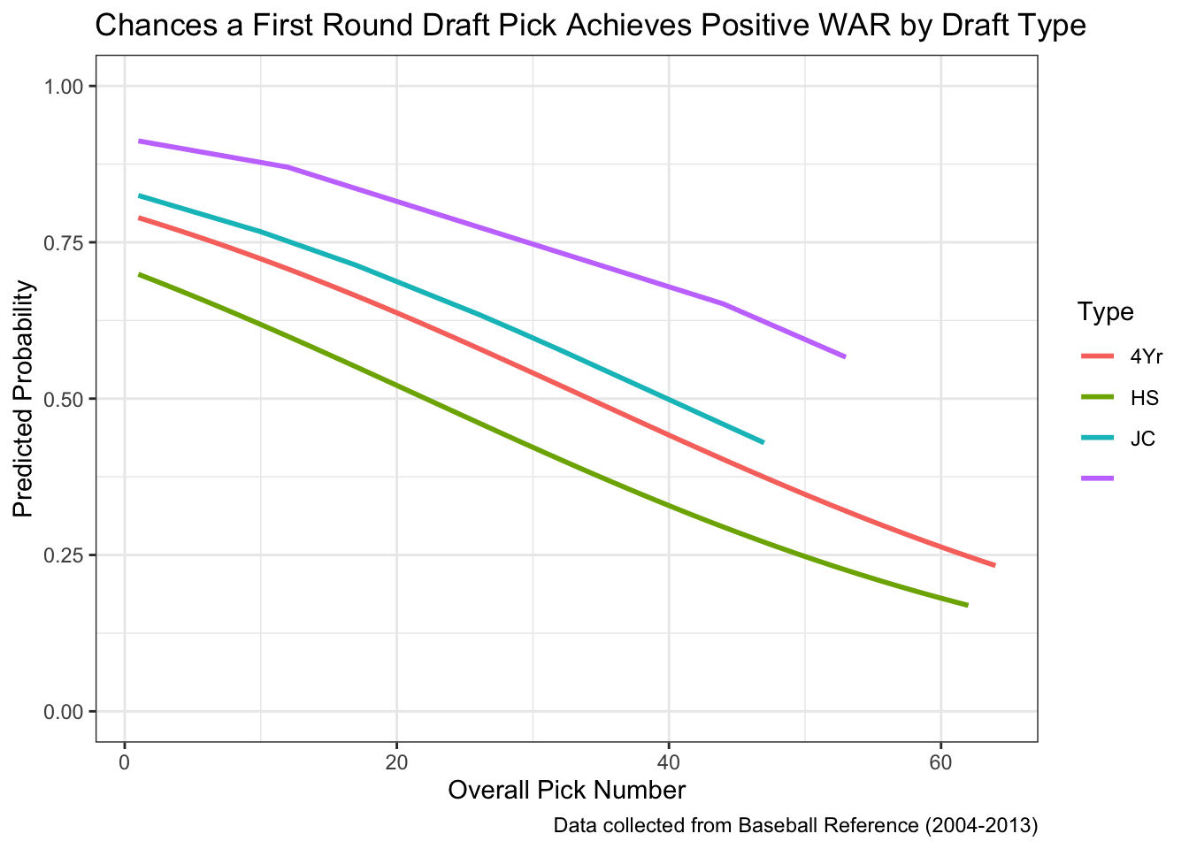
As you can see in the graph, each type has a different predicted probabily even when the overall pick number remains constant. However, we must remain cautious when looking at the “JC” and ” ” types because there are very few observations. Therefore, we should focus only on “4Yr” and “HS”.