R ile Istatiksel Programalama Donem Sonu Odevi
Ozgur Gultekin
knitr::opts_chunk$set(echo = TRUE)R Markdown
Bu R Markdown dokuman R ile Istatistik Programlama Dersi’nin donem sonu odevini sunmak icin hazirlanmistir.
library(tidyverse)## Warning: package 'tidyverse' was built under R version 3.5.3## -- Attaching packages -------------------------------------------------------------------- tidyverse 1.3.0 --## v ggplot2 3.2.1 v purrr 0.3.3
## v tibble 2.1.3 v dplyr 0.8.3
## v tidyr 1.0.0 v stringr 1.4.0
## v readr 1.3.1 v forcats 0.4.0## Warning: package 'ggplot2' was built under R version 3.5.3## Warning: package 'tibble' was built under R version 3.5.3## Warning: package 'tidyr' was built under R version 3.5.3## Warning: package 'readr' was built under R version 3.5.3## Warning: package 'purrr' was built under R version 3.5.3## Warning: package 'dplyr' was built under R version 3.5.3## Warning: package 'forcats' was built under R version 3.5.3## -- Conflicts ----------------------------------------------------------------------- tidyverse_conflicts() --
## x dplyr::filter() masks stats::filter()
## x dplyr::lag() masks stats::lag()library(ggplot2)#Veri dosyadan okunur
myData<-read.csv("avocado.csv")#Verinin ilk 10 satiri goruntulenir
head(myData,10)## X Date AveragePrice Total.Volume X4046 X4225 X4770 Total.Bags
## 1 0 2015-12-27 1.33 64236.62 1036.74 54454.85 48.16 8696.87
## 2 1 2015-12-20 1.35 54876.98 674.28 44638.81 58.33 9505.56
## 3 2 2015-12-13 0.93 118220.22 794.70 109149.67 130.50 8145.35
## 4 3 2015-12-06 1.08 78992.15 1132.00 71976.41 72.58 5811.16
## 5 4 2015-11-29 1.28 51039.60 941.48 43838.39 75.78 6183.95
## 6 5 2015-11-22 1.26 55979.78 1184.27 48067.99 43.61 6683.91
## 7 6 2015-11-15 0.99 83453.76 1368.92 73672.72 93.26 8318.86
## 8 7 2015-11-08 0.98 109428.33 703.75 101815.36 80.00 6829.22
## 9 8 2015-11-01 1.02 99811.42 1022.15 87315.57 85.34 11388.36
## 10 9 2015-10-25 1.07 74338.76 842.40 64757.44 113.00 8625.92
## Small.Bags Large.Bags XLarge.Bags type year region
## 1 8603.62 93.25 0 conventional 2015 Albany
## 2 9408.07 97.49 0 conventional 2015 Albany
## 3 8042.21 103.14 0 conventional 2015 Albany
## 4 5677.40 133.76 0 conventional 2015 Albany
## 5 5986.26 197.69 0 conventional 2015 Albany
## 6 6556.47 127.44 0 conventional 2015 Albany
## 7 8196.81 122.05 0 conventional 2015 Albany
## 8 6266.85 562.37 0 conventional 2015 Albany
## 9 11104.53 283.83 0 conventional 2015 Albany
## 10 8061.47 564.45 0 conventional 2015 Albany#Verinin yapisi incelenir
str(myData)## 'data.frame': 18249 obs. of 14 variables:
## $ X : int 0 1 2 3 4 5 6 7 8 9 ...
## $ Date : Factor w/ 169 levels "2015-01-04","2015-01-11",..: 52 51 50 49 48 47 46 45 44 43 ...
## $ AveragePrice: num 1.33 1.35 0.93 1.08 1.28 1.26 0.99 0.98 1.02 1.07 ...
## $ Total.Volume: num 64237 54877 118220 78992 51040 ...
## $ X4046 : num 1037 674 795 1132 941 ...
## $ X4225 : num 54455 44639 109150 71976 43838 ...
## $ X4770 : num 48.2 58.3 130.5 72.6 75.8 ...
## $ Total.Bags : num 8697 9506 8145 5811 6184 ...
## $ Small.Bags : num 8604 9408 8042 5677 5986 ...
## $ Large.Bags : num 93.2 97.5 103.1 133.8 197.7 ...
## $ XLarge.Bags : num 0 0 0 0 0 0 0 0 0 0 ...
## $ type : Factor w/ 2 levels "conventional",..: 1 1 1 1 1 1 1 1 1 1 ...
## $ year : int 2015 2015 2015 2015 2015 2015 2015 2015 2015 2015 ...
## $ region : Factor w/ 54 levels "Albany","Atlanta",..: 1 1 1 1 1 1 1 1 1 1 ...#year degiskeni factor tipinde degiskene donusturulur.
myData$year<-as.factor(myData$year)#Veriye ait tanimlayici istatistikler incelenir
summary(myData)## X Date AveragePrice Total.Volume
## Min. : 0.00 2015-01-04: 108 Min. :0.440 Min. : 85
## 1st Qu.:10.00 2015-01-11: 108 1st Qu.:1.100 1st Qu.: 10839
## Median :24.00 2015-01-18: 108 Median :1.370 Median : 107377
## Mean :24.23 2015-01-25: 108 Mean :1.406 Mean : 850644
## 3rd Qu.:38.00 2015-02-01: 108 3rd Qu.:1.660 3rd Qu.: 432962
## Max. :52.00 2015-02-08: 108 Max. :3.250 Max. :62505647
## (Other) :17601
## X4046 X4225 X4770 Total.Bags
## Min. : 0 Min. : 0 Min. : 0 Min. : 0
## 1st Qu.: 854 1st Qu.: 3009 1st Qu.: 0 1st Qu.: 5089
## Median : 8645 Median : 29061 Median : 185 Median : 39744
## Mean : 293008 Mean : 295155 Mean : 22840 Mean : 239639
## 3rd Qu.: 111020 3rd Qu.: 150207 3rd Qu.: 6243 3rd Qu.: 110783
## Max. :22743616 Max. :20470573 Max. :2546439 Max. :19373134
##
## Small.Bags Large.Bags XLarge.Bags type
## Min. : 0 Min. : 0 Min. : 0.0 conventional:9126
## 1st Qu.: 2849 1st Qu.: 127 1st Qu.: 0.0 organic :9123
## Median : 26363 Median : 2648 Median : 0.0
## Mean : 182195 Mean : 54338 Mean : 3106.4
## 3rd Qu.: 83338 3rd Qu.: 22029 3rd Qu.: 132.5
## Max. :13384587 Max. :5719097 Max. :551693.7
##
## year region
## 2015:5615 Albany : 338
## 2016:5616 Atlanta : 338
## 2017:5722 BaltimoreWashington: 338
## 2018:1296 Boise : 338
## Boston : 338
## BuffaloRochester : 338
## (Other) :16221#Bölgelerin yıllara göre ortalama satis hacmi tablosu
regional_volume_byYear<-aggregate(x=myData$Total.Volume,by=list(myData$region,myData$year),FUN=mean)
colnames(regional_volume_byYear)<-c("region","year","mean")
regional_volume_byYear[order(regional_volume_byYear$mean,decreasing=T),]## region year mean
## 214 TotalUS 2018 21818010.59
## 160 TotalUS 2017 17591448.71
## 106 TotalUS 2016 17491914.83
## 52 TotalUS 2015 15935146.36
## 215 West 2018 3853211.88
## 208 SouthCentral 2018 3804321.23
## 169 California 2018 3489221.21
## 107 West 2016 3313243.61
## 161 West 2017 3255230.34
## 61 California 2016 3136426.76
## 154 SouthCentral 2017 3070024.68
## 115 California 2017 2996646.49
## 53 West 2015 2929522.30
## 100 SouthCentral 2016 2924025.96
## 7 California 2015 2898148.40
## 46 SouthCentral 2015 2792832.63
## 192 Northeast 2018 2763480.70
## 209 Southeast 2018 2511852.94
## 178 GreatLakes 2018 2215028.25
## 138 Northeast 2017 2119314.16
## 84 Northeast 2016 2105106.59
## 188 Midsouth 2018 2013058.00
## 30 Northeast 2015 1955567.17
## 101 Southeast 2016 1905014.21
## 155 Southeast 2017 1856011.81
## 124 GreatLakes 2017 1786357.23
## 70 GreatLakes 2016 1709038.75
## 16 GreatLakes 2015 1628730.53
## 185 LosAngeles 2018 1585515.73
## 77 LosAngeles 2016 1568675.99
## 134 Midsouth 2017 1561825.95
## 47 Southeast 2015 1539377.01
## 131 LosAngeles 2017 1495105.42
## 80 Midsouth 2016 1483274.02
## 23 LosAngeles 2015 1425198.97
## 26 Midsouth 2015 1348287.66
## 198 Plains 2018 1167836.37
## 191 NewYork 2018 988718.97
## 144 Plains 2017 946038.03
## 90 Plains 2016 915784.94
## 36 Plains 2015 842680.68
## 181 Houston 2018 832604.88
## 174 DallasFtWorth 2018 757156.06
## 196 PhoenixTucson 2018 750533.56
## 137 NewYork 2017 706138.43
## 83 NewYork 2016 687947.72
## 29 NewYork 2015 678919.58
## 127 Houston 2017 651821.63
## 120 DallasFtWorth 2017 624914.93
## 66 DallasFtWorth 2016 612454.33
## 12 DallasFtWorth 2015 579916.43
## 142 PhoenixTucson 2017 577080.51
## 88 PhoenixTucson 2016 570035.45
## 73 Houston 2016 564469.10
## 34 PhoenixTucson 2015 549771.98
## 205 SanFrancisco 2018 540969.14
## 19 Houston 2015 532571.84
## 165 BaltimoreWashington 2018 506620.96
## 175 Denver 2018 493556.39
## 216 WestTexNewMexico 2018 491700.87
## 171 Chicago 2018 483926.32
## 162 WestTexNewMexico 2017 455669.13
## 67 Denver 2016 435651.56
## 108 WestTexNewMexico 2016 421225.30
## 187 MiamiFtLauderdale 2018 405892.53
## 54 WestTexNewMexico 2015 403145.61
## 121 Denver 2017 401500.73
## 97 SanFrancisco 2016 399323.34
## 9 Chicago 2015 398987.66
## 151 SanFrancisco 2017 395014.18
## 57 BaltimoreWashington 2016 393209.64
## 3 BaltimoreWashington 2015 390822.88
## 111 BaltimoreWashington 2017 386939.95
## 117 Chicago 2017 386610.89
## 63 Chicago 2016 380890.73
## 43 SanFrancisco 2015 379286.56
## 13 Denver 2015 376830.23
## 167 Boston 2018 359875.25
## 91 Portland 2016 358764.54
## 98 Seattle 2016 357580.95
## 199 Portland 2018 349907.94
## 145 Portland 2017 348108.06
## 164 Atlanta 2018 342975.94
## 206 Seattle 2018 330878.93
## 152 Seattle 2017 330448.73
## 79 MiamiFtLauderdale 2016 306587.12
## 59 Boston 2016 293954.95
## 133 MiamiFtLauderdale 2017 291322.93
## 113 Boston 2017 288779.93
## 203 Sacramento 2018 286156.24
## 96 SanDiego 2016 282096.64
## 44 Seattle 2015 279395.19
## 204 SanDiego 2018 278077.10
## 213 Tampa 2018 276752.29
## 193 NorthernNewEngland 2018 276507.02
## 195 Philadelphia 2018 273634.87
## 56 Atlanta 2016 272373.83
## 110 Atlanta 2017 271840.75
## 37 Portland 2015 268687.07
## 5 Boston 2015 263990.30
## 150 SanDiego 2017 256549.93
## 42 SanDiego 2015 255631.98
## 176 Detroit 2018 250956.56
## 194 Orlando 2018 246455.79
## 207 SouthCarolina 2018 243170.06
## 25 MiamiFtLauderdale 2015 241985.69
## 2 Atlanta 2015 223381.71
## 95 Sacramento 2016 222336.83
## 149 Sacramento 2017 218796.50
## 139 NorthernNewEngland 2017 213776.33
## 85 NorthernNewEngland 2016 212902.00
## 87 Philadelphia 2016 212577.85
## 41 Sacramento 2015 211351.33
## 141 Philadelphia 2017 210106.08
## 105 Tampa 2016 208468.74
## 33 Philadelphia 2015 200886.73
## 200 RaleighGreensboro 2018 199537.30
## 159 Tampa 2017 193869.22
## 122 Detroit 2017 193513.44
## 31 NorthernNewEngland 2015 193217.56
## 153 SouthCarolina 2017 188386.48
## 184 LasVegas 2018 187234.65
## 180 HartfordSpringfield 2018 186989.19
## 86 Orlando 2016 184757.57
## 68 Detroit 2016 181802.49
## 99 SouthCarolina 2016 179835.17
## 140 Orlando 2017 177466.06
## 14 Detroit 2015 172880.57
## 190 NewOrleansMobile 2018 169331.69
## 201 RichmondNorfolk 2018 166450.96
## 51 Tampa 2015 164726.90
## 130 LasVegas 2017 164470.12
## 179 HarrisburgScranton 2018 162575.49
## 76 LasVegas 2016 162567.44
## 45 SouthCarolina 2015 156210.26
## 146 RaleighGreensboro 2017 151213.66
## 72 HartfordSpringfield 2016 150941.83
## 172 CincinnatiDayton 2018 149928.64
## 22 LasVegas 2015 149446.43
## 170 Charlotte 2018 149412.07
## 189 Nashville 2018 146348.06
## 18 HartfordSpringfield 2015 145790.80
## 126 HartfordSpringfield 2017 144552.87
## 118 CincinnatiDayton 2017 142893.19
## 32 Orlando 2015 141534.39
## 82 NewOrleansMobile 2016 140772.75
## 92 RaleighGreensboro 2016 140075.52
## 136 NewOrleansMobile 2017 135155.68
## 64 CincinnatiDayton 2016 134816.02
## 147 RichmondNorfolk 2017 128744.57
## 71 HarrisburgScranton 2016 126200.23
## 93 RichmondNorfolk 2016 124404.09
## 125 HarrisburgScranton 2017 124003.00
## 38 RaleighGreensboro 2015 123243.60
## 135 Nashville 2017 122062.69
## 28 NewOrleansMobile 2015 121772.19
## 182 Indianapolis 2018 121194.78
## 173 Columbus 2018 118495.83
## 10 CincinnatiDayton 2015 113040.15
## 183 Jacksonville 2018 112850.18
## 116 Charlotte 2017 112222.55
## 39 RichmondNorfolk 2015 112029.60
## 17 HarrisburgScranton 2015 111902.93
## 177 GrandRapids 2018 107060.97
## 211 StLouis 2018 105735.83
## 202 Roanoke 2018 103782.08
## 103 StLouis 2016 102350.73
## 62 Charlotte 2016 101795.39
## 81 Nashville 2016 100953.60
## 119 Columbus 2017 96605.78
## 49 StLouis 2015 95217.07
## 128 Indianapolis 2017 94350.95
## 15 GrandRapids 2015 93662.91
## 75 Jacksonville 2016 93383.04
## 8 Charlotte 2015 91224.46
## 168 BuffaloRochester 2018 88492.42
## 74 Indianapolis 2016 88119.75
## 69 GrandRapids 2016 87950.69
## 65 Columbus 2016 87110.26
## 129 Jacksonville 2017 86729.13
## 157 StLouis 2017 84793.61
## 27 Nashville 2015 83287.66
## 123 GrandRapids 2017 82589.22
## 197 Pittsburgh 2018 79229.99
## 20 Indianapolis 2015 78740.98
## 148 Roanoke 2017 76279.36
## 11 Columbus 2015 75478.67
## 94 Roanoke 2016 73911.70
## 114 BuffaloRochester 2017 73021.75
## 60 BuffaloRochester 2016 69279.92
## 21 Jacksonville 2015 69004.58
## 40 Roanoke 2015 65180.89
## 143 Pittsburgh 2017 64609.70
## 163 Albany 2018 64249.42
## 186 Louisville 2018 61315.04
## 6 BuffaloRochester 2015 56665.72
## 89 Pittsburgh 2016 53040.36
## 210 Spokane 2018 51078.89
## 55 Albany 2016 50618.61
## 166 Boise 2018 50614.98
## 132 Louisville 2017 49623.67
## 109 Albany 2017 49354.55
## 78 Louisville 2016 48810.85
## 156 Spokane 2017 48599.32
## 102 Spokane 2016 48136.22
## 112 Boise 2017 44910.96
## 58 Boise 2016 44745.28
## 35 Pittsburgh 2015 43653.84
## 212 Syracuse 2018 43624.49
## 24 Louisville 2015 41240.42
## 48 Spokane 2015 40208.53
## 1 Albany 2015 38749.00
## 4 Boise 2015 36388.05
## 158 Syracuse 2017 35207.34
## 104 Syracuse 2016 32974.70
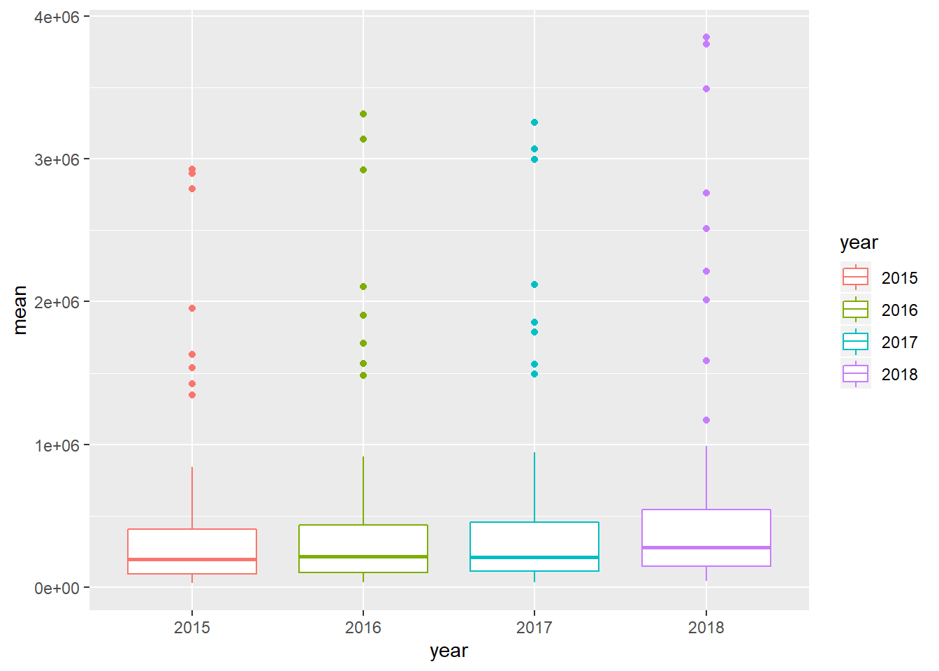
## 50 Syracuse 2015 26291.67#Yillara göre satis hacmi ortalamaları boxplotlari
p <- ggplot(regional_volume_byYear, aes(x=year, y=mean,color=year)) +
geom_boxplot()
p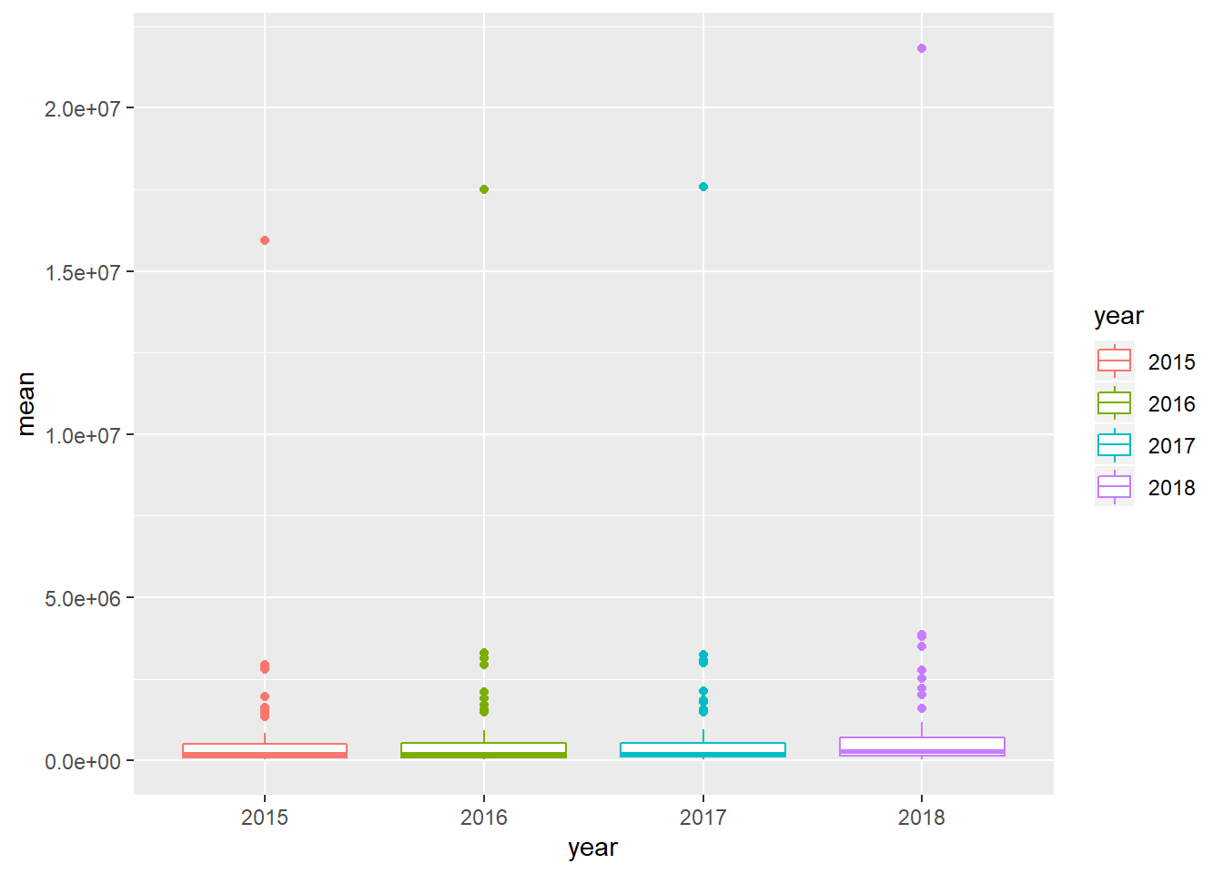
#TotalUS degeri ABD'deki tum bolgeler icin toplam satis hacmini belirtiyor. Bu degerleri veriseitnden
#cikarip tekrar boxplot ciziyoruz
q <- ggplot(regional_volume_byYear[which(regional_volume_byYear$region!="TotalUS"),],
            aes(x=year, y=mean,color=year)) + geom_boxplot()
q