Chapter 5 Quasi-likelihood Methods

5.1 More on Dispersion

Recall the exponential dispersion family:

\[ P(y | \theta, \phi) = \exp \left\{ \frac{y \theta - b(\theta)}{\phi} + c(y, \phi) \right\}. \]

Assume grouping has been taken care of, that is \(\phi_i=\phi/m_i\) and let \(y_i\) be the average response in group \(i\). Then the grouped data distribution is

\[ P(y_i|\theta_i, \phi_i) = \exp \left\{ \frac{y_i\theta_i-b(\theta_i)}{\phi_i} + c(y_i, \phi_i, m_i) \right\}. \]

We already know a basic property:

\[ \mbox{Var}(y_i | \theta_i, \phi_i) = \phi_i \mathcal{V}(\mu_i)= \phi \, \mathcal{V}(\mu_i)/m_i. \]

So, the dispersion \(\phi\) scales the variance of \(y_i\) but does not affect \(E(y_i| \theta_i,\phi_i) = \mu_i = h(\boldsymbol{\beta}^T \boldsymbol{x}_i)\).

We also know that the function \(\mathcal{V}(\mu)\) is characteristic for the response distribution at play, with some examples given in the following table.

\(Y\)	\(\mathcal{V}(\mu)\)	\(\phi\)
\(\mathcal{N}(\mu, \sigma^2)\)	\(1\)	\(\sigma^2\)
\(\mbox{Bernoulli}(p)\)	\(p(1-p)\)	\(1\)
\(\mbox{Poisson}(\mu)\)	\(\mu\)	\(1\)
\(\mbox{Gamma}(\mu, \nu)\)	\(\mu^2\)	\(1/\nu\)
\(IG(\mu, \sigma^2)\)	\(\mu^3\)	\(\sigma^2\)

What is then the relevance of dispersion?

For estimation of \(\boldsymbol{\beta}\), we note from Equations (2.5) and (2.6) that

\[ S(\boldsymbol{\beta}) = \frac{1}{\phi}\sum_{i=1}^n m_i \, \frac{y_i - \mu_i}{\mathcal{V}(\mu_i)} \, h'(\eta_i) \, \boldsymbol{x}_i \stackrel{!}{=}0, \]

where \(\stackrel{!}{=}0\) means we set the left-hand side to zero and solve for \(\boldsymbol\beta\). In this case, \(\phi\) cancels out when setting the score function to 0. Hence, dispersion is irrelevant for the estimation of \(\boldsymbol\beta\).

But for the variance of \(\hat{\boldsymbol\beta}\), using Equation (2.12), we have

\[ \begin{aligned} \mbox{Var}(\hat{\boldsymbol\beta}) &\stackrel{a}{=} [ F_{(\phi)}(\hat{\boldsymbol\beta}) ]^{-1} \\ &= \left[ \frac{1}{\phi} \sum_{i=1}^n m_i \frac{h'(\eta_i)^2}{\mathcal{V}(\mu_i)} \boldsymbol{x}_i \boldsymbol{x}_i^T \right]^{-1} \\ &= \phi \left[ \sum_{i=1}^n m_i \frac{h'(\eta_i)^2}{\mathcal{V}(\mu_i)} \boldsymbol{x}_i \boldsymbol{x}_i^T \right]^{-1} \\ &= \phi \, [ F_{(\phi=1)}(\hat{\boldsymbol\beta}) ]^{-1} \end{aligned} \] where \(F_{(\phi)}(\hat{\boldsymbol\beta})\) is the (expected) Fisher information when using dispersion value \(\phi\).

This result implies that a dispersion of \(\phi\) will inflate all standard errors, \(SE(\hat{\beta}_j)\), by a factor \(\sqrt{\phi}\) when compared to using \(\phi=1\).

Estimation of dispersion

Estimation of dispersion can be motivated through goodness-of-fit statistics.

\(\bullet\) Pearson statistic: With the Pearson goodness-of-fit statistic

\[ \chi^2_P= \sum_{i=1}^n m_i \frac{(y_i-\hat{\mu}_i)^2}{\mathcal{V}(\hat{\mu}_i)}, \]

we know that

\[ \begin{aligned} \chi^2_P &\stackrel{a}{\sim} \phi \chi^2(n-p) \\ E(\chi^2_P) &= \phi \, (n-p), \end{aligned} \]

which suggests

\[ \hat{\phi}_{\text{Pearson}} = \frac{\chi^2_P}{n-p}. \]

\(\bullet\) Deviance statistic: With the deviance

\[ D(\boldsymbol{Y}, \hat{\boldsymbol{\mu}}) = 2 \, \phi \, (\ell_{sat}-\ell(\hat{\boldsymbol\beta})), \]

we can approximate

\[ \begin{aligned} D(\boldsymbol{Y}, \hat{\boldsymbol\mu}) &\stackrel{a}{\sim} \phi \, \chi^2(n-p) \\ E(D(\boldsymbol{Y}, \hat{\boldsymbol\mu})) &= \phi \, (n-p), \end{aligned} \]

which suggests

\[ \hat{\phi}_{\text{dev}} = \frac{D(\boldsymbol{Y}, \hat{\boldsymbol\mu})}{n-p}. \]

The notation \(a\) in the distributional expressions above highlights that these are just approximations. For the deviance, we know that the approximation can be very poor! Therefore, the deviance-based estimate is sometimes called the “quick-and-dirty” dispersion estimate.

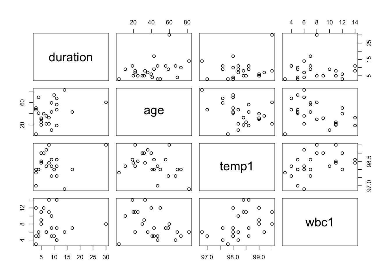
5.1.1 Example: Hospital Stay Data

We consider again the hospital stay data with a Gamma GLM.

require(npmlreg)
data(hosp)
plot(hosp[,c("duration","age","temp1","wbc1")])

hosp.glm <- glm(duration~age+temp1, data=hosp, family=Gamma(link=log))
summary(hosp.glm)

## 
## Call:
## glm(formula = duration ~ age + temp1, family = Gamma(link = log), 
##     data = hosp)
## 
## Coefficients:
##               Estimate Std. Error t value Pr(>|t|)  
## (Intercept) -28.654096  16.621018  -1.724   0.0987 .
## age           0.014900   0.005698   2.615   0.0158 *
## temp1         0.306624   0.168141   1.824   0.0818 .
## ---
## Signif. codes:  0 '***' 0.001 '**' 0.01 '*' 0.05 '.' 0.1 ' ' 1
## 
## (Dispersion parameter for Gamma family taken to be 0.2690233)
## 
##     Null deviance: 8.1722  on 24  degrees of freedom
## Residual deviance: 5.7849  on 22  degrees of freedom
## AIC: 142.73
## 
## Number of Fisher Scoring iterations: 6

We can obtain the dispersion estimate via the Pearson statistic by:

hosp.disp <- 1/(hosp.glm$df.res) * sum((hosp$duration-hosp.glm$fitted)^2/(hosp.glm$fitted^2))
hosp.disp

## [1] 0.2690233

We can also obtain the “quick-and-dirty” dispersion estimate via deviance by:

hosp.glm$deviance/hosp.glm$df.residual

## [1] 0.2629518

The code below extracts the “unscaled” covariance matrix (which is \([ F_{(\phi=1)}(\hat{\boldsymbol\beta}) ]^{-1}\) above) and manually scales the standard errors (the square root of the diagonal) with the square root of the dispersion estimate. The result should be the same as the standard error column in the model summary.

summary(hosp.glm)$cov.unscaled  # F^(-1) under phi=1

##              (Intercept)           age         temp1
## (Intercept) 1026.8932335 -0.1386065114 -10.387121099
## age           -0.1386065  0.0001206901   0.001359292
## temp1        -10.3871211  0.0013592917   0.105088741

sqrt(hosp.disp) * sqrt(diag(summary(hosp.glm)$cov.unscaled)) 

## (Intercept)         age       temp1 
## 16.62101763  0.00569811  0.16814078

summary(hosp.glm)$coef[,"Std. Error"]

## (Intercept)         age       temp1 
## 16.62101763  0.00569811  0.16814078

5.2 Overdispersion

Recall, for the Poisson GLMs, one has \(\phi=1\), i.e.

\[ \mbox{Var}(y_i|\theta_i) = 1 \times \mathcal{V}(\mu_i) = \mathcal{V}(\mu_i) = \mu_i = E(y_i|\theta_i). \]

Thus, \[ \frac{\mbox{Var}(y_i|\theta_i)}{E(y_i|\theta_i)}=1, \] a property referred to as “equidispersion”. This is an assumption of Poisson models, where the mean and variance are assumed to be equal.

5.2.1 Example: US Polio Data

We consider the previous US Polio data, where we fitted a Poisson GLM with a simple linear predictor.

require(gamlss.data)
data(polio)
uspolio <- as.data.frame(matrix(c(1:168, t(polio)), ncol=2))
colnames(uspolio) <- c("time", "cases")

polio.glm <- glm(cases ~ time, family=poisson(link=log), data=uspolio)
summary(polio.glm)

## 
## Call:
## glm(formula = cases ~ time, family = poisson(link = log), data = uspolio)
## 
## Coefficients:
##              Estimate Std. Error z value Pr(>|z|)    
## (Intercept)  0.626639   0.123641   5.068 4.02e-07 ***
## time        -0.004263   0.001395  -3.055  0.00225 ** 
## ---
## Signif. codes:  0 '***' 0.001 '**' 0.01 '*' 0.05 '.' 0.1 ' ' 1
## 
## (Dispersion parameter for poisson family taken to be 1)
## 
##     Null deviance: 343.00  on 167  degrees of freedom
## Residual deviance: 333.55  on 166  degrees of freedom
## AIC: 594.59
## 
## Number of Fisher Scoring iterations: 5

Looking at the summary, we see \(\phi=1\). But let’s get a quick dispersion estimate:

polio.disp <- 333.55/166
polio.disp

## [1] 2.009337

Now with the seasonal model (after adding annual and semi-annual cycles):

polio2.glm <- glm(cases ~ time + I(cos(2*pi*time/12)) + I(sin(2*pi*time/12))
                  + I(cos(2*pi*time/6)) + I(sin(2*pi*time/6)),
                  family=poisson(link=log), data=uspolio)
summary(polio2.glm)

## 
## Call:
## glm(formula = cases ~ time + I(cos(2 * pi * time/12)) + I(sin(2 * 
##     pi * time/12)) + I(cos(2 * pi * time/6)) + I(sin(2 * pi * 
##     time/6)), family = poisson(link = log), data = uspolio)
## 
## Coefficients:
##                           Estimate Std. Error z value Pr(>|z|)    
## (Intercept)               0.557241   0.127303   4.377 1.20e-05 ***
## time                     -0.004799   0.001403  -3.421 0.000625 ***
## I(cos(2 * pi * time/12))  0.137132   0.089479   1.533 0.125384    
## I(sin(2 * pi * time/12)) -0.534985   0.115476  -4.633 3.61e-06 ***
## I(cos(2 * pi * time/6))   0.458797   0.101467   4.522 6.14e-06 ***
## I(sin(2 * pi * time/6))  -0.069627   0.098123  -0.710 0.477957    
## ---
## Signif. codes:  0 '***' 0.001 '**' 0.01 '*' 0.05 '.' 0.1 ' ' 1
## 
## (Dispersion parameter for poisson family taken to be 1)
## 
##     Null deviance: 343.00  on 167  degrees of freedom
## Residual deviance: 288.85  on 162  degrees of freedom
## AIC: 557.9
## 
## Number of Fisher Scoring iterations: 5

The dispersion estimate for this model is:

polio2.disp <- 288.85/162
polio2.disp

## [1] 1.783025

We see that the dispersion reduces when improving the fit of the model, but it is unlikely to “disappear” fully.

In the example above, there is overdispersion, i.e. more dispersion in the data than supported by the model assumption (e.g. \(\phi=1\) in Poisson models).

5.2.2 Reasons and Impacts of Overdispersion

Overdispersion can arise for all one-parameter exponential family distributions (Poisson, Bernoulli/Binomial, etc.). Possible reasons for overdispersion can include:

• Model misspecification (such as omitted covariates);
• Latent clusters/subpopulations in the data (“unobserved heterogeneity”).

What are the impacts of overdispersion?

• There is no impact on \(\hat{\boldsymbol\beta}\).
• The standard error, \(SE(\hat{\beta}_j)\), when estimated using \(\phi=1\), is underestimated by the factor \(\sqrt{\phi}\) (with \(\phi\) denoting the “true” dispersion in the data).

As a consequence,

• Confidence intervals will be too small;
• p-values will be too small;
• Hence, significances are overstated and potentially leading to wrong decisions.

5.3 Quasi-likelihood Methods

Fortunately, there is a simple remedy to the above overdispersion problem, where we can do the following steps:

1. Fit a Poisson or Bernoulli/Binomial model as usual.
2. Estimate \(\phi\) as discussed above, yielding \(\hat{\phi}\).
3. Manually multiply all standard errors by \(\sqrt{\hat{\phi}}\).

De facto, this amounts to the model:

\[ \begin{aligned} \mu_i = h(\boldsymbol\beta^T \boldsymbol{x}_i)\\ \mbox{Var}(y_i)= \phi \, \mathcal{V}(\mu_i), \end{aligned} \] where \(\phi\) is now allowed to vary to capture the actual dispersion in the data.

The score function of this model is called the “quasi-score function” and has the following form, in which clearly \(\phi\) cancels out when estimating \(\boldsymbol\beta\):

\[ S(\boldsymbol\beta) = \sum_{i=1}^n m_i \frac{y_i-\mu_i}{\phi \, \mathcal{V}(\mu_i)} h'(\eta_i) ~ \boldsymbol{x}_i \stackrel{!}{=}0 \]

The variance estimate of \(\hat{\boldsymbol\beta}\) is:

\[ \widehat{\text{Var}}(\hat{\boldsymbol\beta}) = \hat{\phi} \, F^{-1}(\hat{\boldsymbol\beta}). \]

Note that the expressions for \(S(\boldsymbol\beta)\) and \(\widehat{\text{Var}}(\hat{\boldsymbol\beta})\) above are similar to those of the normal GLMs, except for the value of \(\hat{\phi}\), which may be different from the theoretical value. Additionally, doing all this requires no actual distributional assumption (and there could also not be any: The “Poisson”-type EDF with \(\phi>1\) is not a valid pdf!)

Estimation methods using the quasi-score function above are also referred to as quasi-likelihood methods.

5.3.1 Example: US Polio Data

First, let us produce the Pearson-type dispersion estimates for polio.glm and polio2.glm.

polio.phi <- 1/(polio.glm$df.res) * sum((uspolio$cases-polio.glm$fitted)^2/(polio.glm$fitted))
polio.phi

## [1] 2.481818

polio2.phi <- 1/(polio2.glm$df.res) * sum((uspolio$cases-polio2.glm$fitted)^2/(polio2.glm$fitted))
polio2.phi

## [1] 1.967417

Note that these estimates are larger than the assumed value \(1\) of the Poisson family, and thus there are overdispersion in both models. We can then adjust the standard errors manually:

polio.se <- sqrt(polio.phi)*summary(polio.glm)$coef[,2]
polio.se

## (Intercept)        time 
## 0.194781773 0.002198181

polio2.se <- sqrt(polio2.phi)*summary(polio2.glm)$coef[,2]
polio2.se 

##              (Intercept)                     time I(cos(2 * pi * time/12)) 
##              0.178560577              0.001967754              0.125507133 
## I(sin(2 * pi * time/12))  I(cos(2 * pi * time/6))  I(sin(2 * pi * time/6)) 
##              0.161971821              0.142321901              0.137631208

These results can be obtained in R directly through the use of the quasipoisson (or, similarly, quasibinomial) family:

polio.qglm <- glm(cases ~ time, family=quasipoisson(link=log), data=uspolio)
summary(polio.qglm)

## 
## Call:
## glm(formula = cases ~ time, family = quasipoisson(link = log), 
##     data = uspolio)
## 
## Coefficients:
##              Estimate Std. Error t value Pr(>|t|)   
## (Intercept)  0.626639   0.194788   3.217  0.00156 **
## time        -0.004263   0.002198  -1.939  0.05415 . 
## ---
## Signif. codes:  0 '***' 0.001 '**' 0.01 '*' 0.05 '.' 0.1 ' ' 1
## 
## (Dispersion parameter for quasipoisson family taken to be 2.481976)
## 
##     Null deviance: 343.00  on 167  degrees of freedom
## Residual deviance: 333.55  on 166  degrees of freedom
## AIC: NA
## 
## Number of Fisher Scoring iterations: 5

polio2.qglm <- glm(cases ~ time + I(cos(2*pi*time/12)) + I(sin(2*pi*time/12))
                   + I(cos(2*pi*time/6)) + I(sin(2*pi*time/6)),
                   family=quasipoisson(link=log), data=uspolio)
summary(polio2.qglm)

## 
## Call:
## glm(formula = cases ~ time + I(cos(2 * pi * time/12)) + I(sin(2 * 
##     pi * time/12)) + I(cos(2 * pi * time/6)) + I(sin(2 * pi * 
##     time/6)), family = quasipoisson(link = log), data = uspolio)
## 
## Coefficients:
##                           Estimate Std. Error t value Pr(>|t|)   
## (Intercept)               0.557241   0.178566   3.121  0.00214 **
## time                     -0.004799   0.001968  -2.439  0.01583 * 
## I(cos(2 * pi * time/12))  0.137132   0.125511   1.093  0.27620   
## I(sin(2 * pi * time/12)) -0.534985   0.161977  -3.303  0.00118 **
## I(cos(2 * pi * time/6))   0.458797   0.142326   3.224  0.00153 **
## I(sin(2 * pi * time/6))  -0.069627   0.137635  -0.506  0.61363   
## ---
## Signif. codes:  0 '***' 0.001 '**' 0.01 '*' 0.05 '.' 0.1 ' ' 1
## 
## (Dispersion parameter for quasipoisson family taken to be 1.96754)
## 
##     Null deviance: 343.00  on 167  degrees of freedom
## Residual deviance: 288.85  on 162  degrees of freedom
## AIC: NA
## 
## Number of Fisher Scoring iterations: 5

Testing for Overdispersion

Using the fact that \(\hat{\phi}_{\text{Pearson}} = \chi^2_P/(n-p)\) and \(\chi^2_P \stackrel{a}{\sim} \chi^2(n-p)\) under the null hypothesis \(H_0\): \(\phi=1\), one can test for the presence of overdispersion by comparing \(\hat{\phi}_{\text{Pearson}}\) to \(\chi^2_{n-p,\alpha}/(n-p)\).

For instance, for the two Poisson models polio.glm and polio2.glm above, the critical values for \(H_0\): \(\phi=1\) at the \(5\%\) level of significance would be:

qchisq(0.95, polio.glm$df.res)/polio.glm$df.res

## [1] 1.187132

qchisq(0.95, polio2.glm$df.res)/polio2.glm$df.res

## [1] 1.189507

Thus, \(H_0\) would be rejected in both cases.

5.4 Generalized Estimating Equations

The quasi-likelihood techniques discussed in the previous subsection motivate a more general concept. First, we rewrite the score function into matrix form (see Section 2.7.1):

\[ S(\boldsymbol\beta) = \sum_{i=1}^n \frac{y_i-\mu_i}{\phi_i \, \mathcal{V}(\mu_i)}h'(\eta_i) \, \boldsymbol{x}_i = \boldsymbol{X}^T \boldsymbol{D} \boldsymbol{\Sigma}^{-1} (\boldsymbol{Y}-\boldsymbol{\mu}) \]

where as usual:

\[ \begin{aligned} \phi_i &= \phi/m_i \\ \eta_i &= \boldsymbol\beta^T \boldsymbol{x}_i \\ \boldsymbol{D} &= \mbox{diag}(h'(\eta_i)) \\ \boldsymbol\Sigma &= \mbox{diag}(\mbox{Var}(y_i)) = \mbox{diag}(\phi_i \, \mathcal{V}(\mu_i)). \end{aligned} \]

The idea is now to replace the matrix \(\boldsymbol\Sigma\) (the shape of which was originally motivated directly by GLM properties) by any appropriate “working covariance” matrix \(\boldsymbol\Sigma = \mbox{Var}(\boldsymbol{Y})\), in this manner trying to capture any correlation structures in the data as correctly as possible. From here, we would compute (just as for GLMs):

\[ F(\boldsymbol\beta) = \boldsymbol{X}^T \boldsymbol{D}^T \boldsymbol\Sigma^{-1} \boldsymbol{D} \boldsymbol{X}, \]

allowing us to estimate the variance of \(\hat{\boldsymbol\beta}\) as

\[ \mbox{Var}(\hat{\boldsymbol\beta}) \approx F^{-1}(\hat{\boldsymbol\beta}). \]

This general technique is called Generalized Estimating Equations (GEEs). Note that the quasi-likelihood method is a special case of GEEs since the matrix \(\boldsymbol\Sigma\) in the quasi-likelihood method varies only through the value of \(\phi\).

Important theoretical result: Under some regularity conditions, the estimator \(\hat{\boldsymbol\beta}\) is consistent and asymptotically normal even if \(\boldsymbol\Sigma\) is wrong!

5.4.1 Example: US Polio Data

We first use GEEs to provide an equivalent estimate of the quasipoisson approach. Below, the argument id=rep(1,168) means all data points are in the same cluster and the argument corstr = "independence" means that data points in each cluster are independent. So, basically this is just the usual independent data assumption. We will see this in more detail in the next chapter.

require(gee)

## Loading required package: gee

uspolio.gee <- gee(cases ~ time 
                   + I(cos(2*pi*time/12)) + I(sin(2*pi*time/12))
                   + I(cos(2*pi*time/6)) + I(sin(2*pi*time/6)),
                   family=poisson(link=log), id=rep(1,168),
                   corstr = "independence", data=uspolio)

## Beginning Cgee S-function, @(#) geeformula.q 4.13 98/01/27

## running glm to get initial regression estimate

##              (Intercept)                     time I(cos(2 * pi * time/12)) 
##              0.557240558             -0.004798661              0.137131634 
## I(sin(2 * pi * time/12))  I(cos(2 * pi * time/6))  I(sin(2 * pi * time/6)) 
##             -0.534985461              0.458797164             -0.069627044

uspolio.gee

## 
##  GEE:  GENERALIZED LINEAR MODELS FOR DEPENDENT DATA
##  gee S-function, version 4.13 modified 98/01/27 (1998) 
## 
## Model:
##  Link:                      Logarithm 
##  Variance to Mean Relation: Poisson 
##  Correlation Structure:     Independent 
## 
## Call:
## gee(formula = cases ~ time + I(cos(2 * pi * time/12)) + I(sin(2 * 
##     pi * time/12)) + I(cos(2 * pi * time/6)) + I(sin(2 * pi * 
##     time/6)), id = rep(1, 168), data = uspolio, family = poisson(link = log), 
##     corstr = "independence")
## 
## Number of observations :  168 
## 
## Maximum cluster size   :  168 
## 
## 
## Coefficients:
##              (Intercept)                     time I(cos(2 * pi * time/12)) 
##              0.557240556             -0.004798661              0.137131637 
## I(sin(2 * pi * time/12))  I(cos(2 * pi * time/6))  I(sin(2 * pi * time/6)) 
##             -0.534985464              0.458797164             -0.069627041 
## 
## Estimated Scale Parameter:  1.967417
## Number of Iterations:  1
## 
## Working Correlation[1:4,1:4]
##      [,1] [,2] [,3] [,4]
## [1,]    1    0    0    0
## [2,]    0    1    0    0
## [3,]    0    0    1    0
## [4,]    0    0    0    1
## 
## 
## Returned Error Value:
## [1] 0

summary(uspolio.gee)$coef

##                              Estimate Naive S.E.    Naive z  Robust S.E.
## (Intercept)               0.557240556  0.1785640  3.1206774 1.166422e-16
## time                     -0.004798661  0.0019678 -2.4385923 4.904902e-18
## I(cos(2 * pi * time/12))  0.137131637  0.1255114  1.0925831 1.219796e-16
## I(sin(2 * pi * time/12)) -0.534985464  0.1619769 -3.3028513 4.739094e-16
## I(cos(2 * pi * time/6))   0.458797164  0.1423255  3.2235766 2.333805e-16
## I(sin(2 * pi * time/6))  -0.069627041  0.1376347 -0.5058827 4.818703e-17
##                               Robust z
## (Intercept)               4.777351e+15
## time                     -9.783399e+14
## I(cos(2 * pi * time/12))  1.124218e+15
## I(sin(2 * pi * time/12)) -1.128877e+15
## I(cos(2 * pi * time/6))   1.965876e+15
## I(sin(2 * pi * time/6))  -1.444933e+15

But then, there is very likely serial correlation in the data! So, we may try to assume an AR(1) correlation structure within each cluster by specifying corstr="AR-M" and Mv=1.

uspolio.gee2 <- gee(cases ~ time 
                    + I(cos(2*pi*time/12)) + I(sin(2*pi*time/12)) 
                    + I(cos(2*pi*time/6)) + I(sin(2*pi*time/6)),
                    family=poisson(link=log), id=rep(1,168), 
                    data=uspolio, corstr="AR-M", Mv=1)

However, the code above does not fit since the sequence is too long!

We can try to simplify the model. For instance, let us assume we have an AR(1) correlation structure within each year, but different years are independent. To do this, we create the id argument as follows.

id = rep(1:14, each=12)
id

##   [1]  1  1  1  1  1  1  1  1  1  1  1  1  2  2  2  2  2  2  2  2  2  2  2  2  3
##  [26]  3  3  3  3  3  3  3  3  3  3  3  4  4  4  4  4  4  4  4  4  4  4  4  5  5
##  [51]  5  5  5  5  5  5  5  5  5  5  6  6  6  6  6  6  6  6  6  6  6  6  7  7  7
##  [76]  7  7  7  7  7  7  7  7  7  8  8  8  8  8  8  8  8  8  8  8  8  9  9  9  9
## [101]  9  9  9  9  9  9  9  9 10 10 10 10 10 10 10 10 10 10 10 10 11 11 11 11 11
## [126] 11 11 11 11 11 11 11 12 12 12 12 12 12 12 12 12 12 12 12 13 13 13 13 13 13
## [151] 13 13 13 13 13 13 14 14 14 14 14 14 14 14 14 14 14 14

Then we fit the GEE (you can ignore the printed initial regression estimate):

uspolio.gee3 <- gee(cases ~ time 
                    + I(cos(2*pi*time/12)) + I(sin(2*pi*time/12))
                    + I(cos(2*pi*time/6)) + I(sin(2*pi*time/6)),
                    family=poisson(link=log), id=id, 
                    data=uspolio, corstr="AR-M", Mv=1)

## Beginning Cgee S-function, @(#) geeformula.q 4.13 98/01/27

## running glm to get initial regression estimate

##              (Intercept)                     time I(cos(2 * pi * time/12)) 
##              0.557240558             -0.004798661              0.137131634 
## I(sin(2 * pi * time/12))  I(cos(2 * pi * time/6))  I(sin(2 * pi * time/6)) 
##             -0.534985461              0.458797164             -0.069627044

We can look at the model summary and the working correlation matrix:

uspolio.gee3

## 
##  GEE:  GENERALIZED LINEAR MODELS FOR DEPENDENT DATA
##  gee S-function, version 4.13 modified 98/01/27 (1998) 
## 
## Model:
##  Link:                      Logarithm 
##  Variance to Mean Relation: Poisson 
##  Correlation Structure:     AR-M , M = 1 
## 
## Call:
## gee(formula = cases ~ time + I(cos(2 * pi * time/12)) + I(sin(2 * 
##     pi * time/12)) + I(cos(2 * pi * time/6)) + I(sin(2 * pi * 
##     time/6)), id = id, data = uspolio, family = poisson(link = log), 
##     corstr = "AR-M", Mv = 1)
## 
## Number of observations :  168 
## 
## Maximum cluster size   :  12 
## 
## 
## Coefficients:
##              (Intercept)                     time I(cos(2 * pi * time/12)) 
##              0.534670137             -0.004504214              0.127605025 
## I(sin(2 * pi * time/12))  I(cos(2 * pi * time/6))  I(sin(2 * pi * time/6)) 
##             -0.518732586              0.434976179             -0.059598999 
## 
## Estimated Scale Parameter:  1.983319
## Number of Iterations:  3
## 
## Working Correlation[1:4,1:4]
##            [,1]       [,2]       [,3]       [,4]
## [1,] 1.00000000 0.26087713 0.06805688 0.01775448
## [2,] 0.26087713 1.00000000 0.26087713 0.06805688
## [3,] 0.06805688 0.26087713 1.00000000 0.26087713
## [4,] 0.01775448 0.06805688 0.26087713 1.00000000
## 
## 
## Returned Error Value:
## [1] 0

round(summary(uspolio.gee3)$working.correlation, digits=3)

##        [,1]  [,2]  [,3]  [,4]  [,5]  [,6]  [,7]  [,8]  [,9] [,10] [,11] [,12]
##  [1,] 1.000 0.261 0.068 0.018 0.005 0.001 0.000 0.000 0.000 0.000 0.000 0.000
##  [2,] 0.261 1.000 0.261 0.068 0.018 0.005 0.001 0.000 0.000 0.000 0.000 0.000
##  [3,] 0.068 0.261 1.000 0.261 0.068 0.018 0.005 0.001 0.000 0.000 0.000 0.000
##  [4,] 0.018 0.068 0.261 1.000 0.261 0.068 0.018 0.005 0.001 0.000 0.000 0.000
##  [5,] 0.005 0.018 0.068 0.261 1.000 0.261 0.068 0.018 0.005 0.001 0.000 0.000
##  [6,] 0.001 0.005 0.018 0.068 0.261 1.000 0.261 0.068 0.018 0.005 0.001 0.000
##  [7,] 0.000 0.001 0.005 0.018 0.068 0.261 1.000 0.261 0.068 0.018 0.005 0.001
##  [8,] 0.000 0.000 0.001 0.005 0.018 0.068 0.261 1.000 0.261 0.068 0.018 0.005
##  [9,] 0.000 0.000 0.000 0.001 0.005 0.018 0.068 0.261 1.000 0.261 0.068 0.018
## [10,] 0.000 0.000 0.000 0.000 0.001 0.005 0.018 0.068 0.261 1.000 0.261 0.068
## [11,] 0.000 0.000 0.000 0.000 0.000 0.001 0.005 0.018 0.068 0.261 1.000 0.261
## [12,] 0.000 0.000 0.000 0.000 0.000 0.000 0.001 0.005 0.018 0.068 0.261 1.000

This last assumption on the correlation structure of the data leads us to repeated measures data, which is the actual strength of GEEs.

5.5 Exercises

Question 1

1. Explain the phenomenon of overdispersion in a statistical model.
2. For the GLMs in Exercise 3 of Chapter 1, which of them may have overdispersion? Explain your answer.
3. Conduct hypothesis tests to determine whether there is overdispersion in the models polio1.glm and polio3.glm in Section 2.9.

Question 2

Consider again the US Polio data in Section 2.9 and the pairs of models in Exercise 2 of Chapter 3.

1. Perform again the analysis of deviance for these pairs of models using a single anova table of model polio3.glm, but now with the estimated dispersion of the bigger model in each pair.
2. Now instead of fitting Poisson models, we can fit quasi-Poisson models polio.quasi, polio1.quasi, polio2.quasi, and polio3.quasi (which corresponds to polio.glm, polio1.glm, polio2.glm, and polio3.glm). Using the anova command between two quasi-Poisson models, check that your p-values in part (a) are correct.
3. Compare your p-values obtained from part (a) with the p-values obtained in Exercise 2 of Chapter Chapter 4 and the p-values obtained from the Wald tests in Exercise 2 of Chapter 3. Explain any differences in these values.

Question 3

Consider a poll of \(m\) individuals that asked whether they supported a certain government policy. Let \(Y\) be the random variable representing the number of respondents who gave an affirmative answer. We know that \(Y = \sum_{i=1}^m Y_i\), where \(Y_i \sim \text{Bernoulli}(p)\) is the random variable representing the response of the \(i\)-th respondent. Suppose you use a binomial distribution to model \(Y\) such that \(Y \sim \text{Bin}(m, p)\).

1. Assume that the responses are independent and the correlation \(\text{Corr}(Y_i, Y_j) = \tau\) for all \(i, j\). Show that if \(\tau > 0\), then there will be overdispersion in your binomial model.
2. Comment on the case where \(\tau < 0\). Which scenario would make this case happen in a real poll?
3. Now suppose that \(m\) is unknown, but you know that the number of participants in the poll is a random variable \(M\) with mean \(\mu_M\) and variance \(\sigma_M^2\). Assume that \(\mu_M\) and \(\sigma_M\) are both known and \(\mu_M\) is a positive integer number. If you model \(Y\) using the binomial distribution \(\text{Bin}(\mu_M, p)\), find the condition for \(\tau\) such that there is overdispersion in your binomial model.

Question 4

As part of a retrospective chart review of antibiotic use in hospitals, we are provided with data on \(n = 25\) persons discharged from a selected Pennsylvania hospital. The variables in the data set are as follows:

• \({\tt duration}\): response, the total number of days patients spent in hospital.
• \({\tt age}\): age of patient in whole years.
• \({\tt sex}\): gender, \(1 = \text{M}\), \(2 = \text{F}\).
• \({\tt temp1}\): first temperature following admission.
• \({\tt wbc1}\): first white blood cell (WBC) count (\(\times10^3\)) following admission.
• \({\tt antib}\): received antibiotic: \(1 = \text{yes}\), \(2 = \text{no}\).
• \({\tt bact}\): received bacterial culture: \(1 = \text{yes}\), \(2 = \text{no}\).
• \({\tt serv}\): service, \(1 = \text{medical}\), \(2 = \text{surgical}\).

We fit a generalized linear model with Gamma response and log-link to the data, using all available predictor variables. The corresponding R code and output is shown below. The variables will collectively be denoted by \(x\in\mathbb{R}^8\), where \(x_{1}\equiv 1\), with \(x_{2}, \dotsc, x_{8}\) corresponding to the variables in the order listed above. Let \(\beta\in\mathbb{R}^8\) be the corresponding model parameters.

(a)

1. For a gamma distribution, viewed as an EDF, the function \(b(\theta) = -\ln(-\theta)\). Derive the expression for the mean \(\mu\) of the distribution in terms of \(\theta\).

2. Using the standard form for an EDF, write down the log-likelihood function \(\ell(\beta)\) for data \(\{(x_{i}, y_{i})_{i\in[1..n]}\}\), in terms of the means \(\mu_{i}\) of the distributions corresponding to the \(x_{i}\). You do not have to give the explicit form of terms that do not depend on \(\beta\).

3. Derive the expression for the log-likelihood of the saturated model.

4. Derive the expression for the deviance of the original model.

(b) Using the provided value of the deviance of the full model, show that a rough estimate of the dispersion is given by \(\hat{\phi}=0.30\). Use this estimate in all further calculations if required.

(c) We are interested in testing hypotheses of type \(H_{0}: C\beta = 0\) versus \(H_{1}: C\beta \neq 0\). Give the matrix \(C\) corresponding to the test problems:

1. \(H_0: \beta_2=0,\, \beta_3=0\)
2. \(H_0: \beta_6=\beta_7 + \beta_8\)
3. \(H_0: \beta_j=0,\, j=2,\dotsc, 8\)

(d) For item (c.i), carry out, at the \(5\%\) level of significance:

1. A Wald test;
2. A likelihood ratio test.

In each case, explain your steps clearly and justify any distributional assumptions.

Hint: In order to solve (d.ii), work with the deviances of the reduced models given at the bottom of the R excerpt. You do not need the result of part (a.iv) in order to answer this question.

> hosp.full.glm <- glm(duration ~ age + sex + temp1 + wbc1 +
                       antib + bact + serv, data = hosp, family=Gamma(link=log))

> hosp.full.glm

Call:  glm(formula = duration ~ age + sex + temp1 + wbc1 + antib
    + bact + serv, family = Gamma(link = log), data = hosp)

Coefficients:
(Intercept)          age          sex        temp1         wbc1
 -1.844e+01    9.675e-03    5.091e-02    2.139e-01   -2.352e-04
        antib       bact         serv
   -3.756e-01  7.502e-02   -2.802e-01

Degrees of Freedom: 24 Total (i.e. Null);  17 Residual
Null Deviance:      8.172
Residual Deviance: 5.109    AIC: 149.5

> summary(hosp.full.glm)$cov.scaled
             (Intercept)           age           sex         temp1
(Intercept) 339.87206809 -3.874572e-02  0.8075732242 -3.4544034796
age          -0.03874572  4.767174e-05 -0.0001699029  0.0003450604
sex           0.80757322 -1.699029e-04  0.0660872869 -0.0088972055
temp1        -3.45440348  3.450604e-04 -0.0088972055  0.0352421720
wbc1          0.19550988  9.139414e-05 -0.0025269325 -0.0022653901
antib        -0.73456895  3.952404e-04 -0.0288981629  0.0061731593
bact          0.07513739  5.674694e-04 -0.0007987594 -0.0028022084
serv         -0.20040916  4.435970e-04  0.0255644438  0.0009390817
                     wbc1         antib          bact          serv
(Intercept)  1.955099e-01 -0.7345689536  0.0751373872 -0.2004091599
age          9.139414e-05  0.0003952404  0.0005674694  0.0004435970
sex         -2.526933e-03 -0.0288981629 -0.0007987594  0.0255644438
temp1       -2.265390e-03  0.0061731593 -0.0028022084  0.0009390817
wbc1         2.261973e-03  0.0039716337  0.0061319158 -0.0048708786
antib        3.971634e-03  0.0755296413  0.0050162417 -0.0081693577
bact         6.131916e-03  0.0050162417  0.0844887445 -0.0165954896
serv        -4.870879e-03 -0.0081693577 -0.0165954896  0.0800990768
>  glm(duration~age+temp1+wbc1+antib+bact+serv, data=hosp,
    family=Gamma(link=log))$dev
[1] 5.120007
>  glm(duration~temp1+wbc1+antib+bact+serv, data=hosp,
    family=Gamma(link=log))$dev
[1] 5.604124