7 Application: Optimizing catalysis conditions
The following example is a detailed description on how modeling, DoE & optimization has helped to substantially improve the reaction conditions of a catalytic system for converting CO2 to formaldehyde [for details (Siebert M., Krennrich G., Seibicke M., Siegle A.F., Trapp O. 2019)]. The experimental data for reproducing the modeling results with the R code below can be downloaded here. The R-code combines elements from machine learning (here: the Random Forest), experimental design (here: D-optimal design), optimization (here: augmented Lagrange) and relaxation (here: hypercubical relaxation). A visual overview of the optimization course is given in figure 7.1.
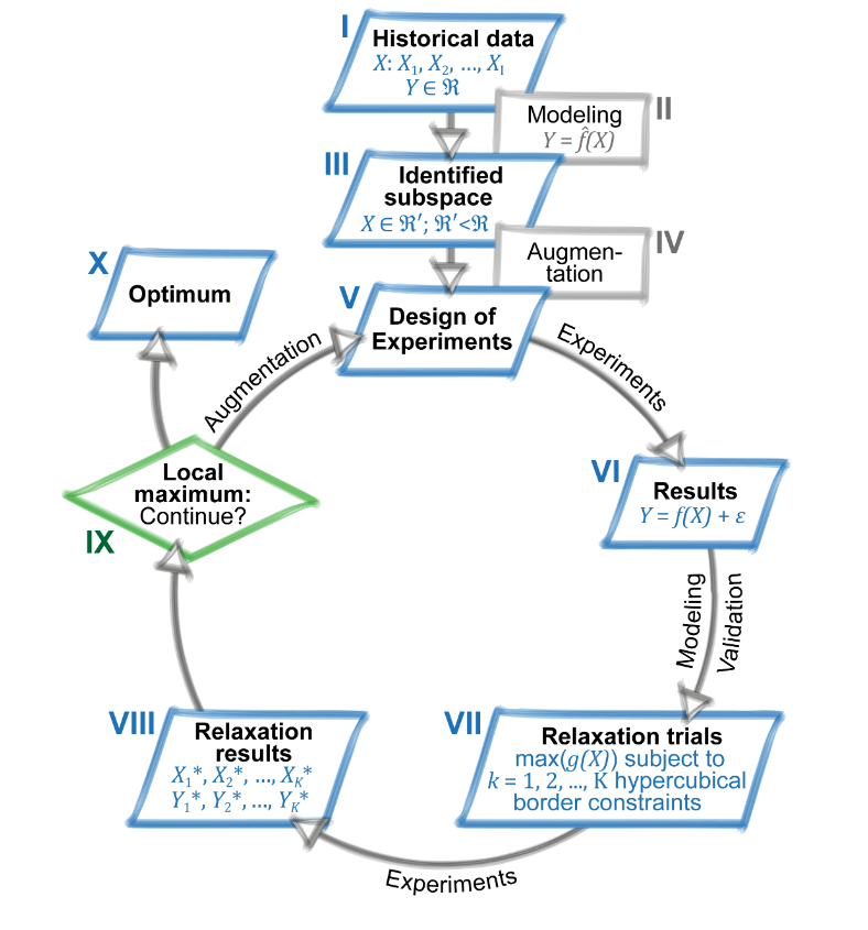
Figure 7.1: Outline of the optimization project
For the optimization project, seven different factors (X-variables) are considered - namely:
- the temperature (T [\(^\textrm{o} \textrm{C}\)]),
- the partial pressure of hydrogen gas (p.h2 [bar]),
- the partial pressure of carbon dioxide gas (p.co2 [bar]),
- the time (t.h [h]),
- the amount of catalyst (m.kat [\(\mu\textrm{mol}\)]),
- the amount of additive Al(OTf)3 (m.add [\(\mu\textrm{mol}\)])
- and the volume of the catalysis solution (v.ml [ml]).
There are two responses (Y-variables) to be maximized over the seven process factors above - namely:
- the turnover number of the main product dimethoxymethane (DMM), abbreviated ton.dmm
- the turnover number of the by-product methyl formate (MF), abbreviated ton.mf
In the following, only the abbreviations mentioned in bold in the brackets are used to refer to the process parameters and responses. The use of units is omitted for the sake of clarity.
The R-code can be run by pasting code chunks (in the grey boxes) to and excecuting them in R-Studio.
Sequential run order is important as subsequent code might depend on objects created by previous code.
7.1 Modelling historical data with the Random Forest (I - III in figure 7.1)
File location: Must be adjusted by the user
input <- file.path("C:","users","myname","data","r.example","c9sc04591k1.xlsx")Next load the required libraries and identify the names of the X- and Y-variables, respectively
library(lattice)
library(randomForest)
library(pals)
library(readxl)
set.seed(12345)
##Read historical data 144 x 10 into data frame x
x.historical <- as.data.frame(read_excel(input,
              sheet="historical.data"))
dim(x.historical) # 144 x 10
## [1] 144 10x.var <- colnames(x.historical)[2:8]
y.var <- colnames(x.historical)[9:10]
xx.historical <- round(x.historical[,c("obsnr",x.var,y.var)],3)| obsnr | m.kat | v.ml | m.add | T | p.h2 | p.co2 | t.h | ton.dmm | ton.mf | |
|---|---|---|---|---|---|---|---|---|---|---|
| 1 | 1 | 1.5 | 0.5 | 6.25 | 20 | 60 | 20 | 18 | 3.856 | 48.735 |
| 2 | 2 | 1.5 | 0.5 | 6.25 | 20 | 60 | 20 | 18 | 7.377 | 45.773 |
| 3 | 3 | 1.5 | 0.5 | 6.25 | 20 | 60 | 20 | 18 | 12.826 | 58.683 |
| 4 | 4 | 1.5 | 0.5 | 6.25 | 70 | 60 | 20 | 18 | 154.421 | 164.816 |
| 5 | 5 | 1.5 | 0.5 | 6.25 | 70 | 60 | 20 | 18 | 155.679 | 162.916 |
| 6 | 6 | 1.5 | 0.5 | 6.25 | 70 | 60 | 20 | 18 | 181.080 | 155.651 |
| 7 | 7 | 1.5 | 0.5 | 6.25 | 80 | 60 | 20 | 18 | 268.602 | 108.201 |
| 8 | 8 | 1.5 | 0.5 | 6.25 | 80 | 60 | 20 | 18 | 289.141 | 114.908 |
| 9 | 9 | 1.5 | 0.5 | 6.25 | 80 | 60 | 20 | 18 | 318.818 | 113.902 |
| 10 | 10 | 1.5 | 0.5 | 6.25 | 85 | 60 | 20 | 18 | 314.123 | 96.297 |
X-variables are located at position 2-8, Y-variables at position 9-10 (step I in figure 7.1).
Do Random-Forest modeling (see (T. Hastie, R. Tibshirani, J. Friedman 2009, 587–604)) and store models as list rf.models().
Report Goodness-of-fit parameter \(R^2\)
rf.models <- list()
R2        <- NULL
for (i in (1:length(y.var)) )   {
# rf modeling; add models to list rf.models
  rf.models[[i]] <- randomForest(
    formula(paste(y.var[i],"~",paste(x.var,collapse="+"),
            sep="")),data=x.historical)
  R2     <- c(R2, round(cor(predict(rf.models[[i]]),
                  x.historical[,y.var[i]])^2,2))
}
names(R2) <- y.var
R2 # show fit in terms of R2
## ton.dmm ton.mf
## 0.83 0.74The Random Forest fits the data well with \(R^2_{ton.dmm}\)=0.83 and \(R^2_{ton.mf}\)=0.74.
Next report some graphical diagnostics by plotting observed versus predicted values of ton.dmm with the observation# used as plot label, see figure 7.2.
plot(predict(rf.models[[1]]), x.historical$ton.dmm,type="n",
     xlab="predicted ton.dmm", ylab="observed ton.dmm")
text(predict(rf.models[[1]]),
     x.historical$ton.dmm,labels=x.historical$obsnr)
abline(0,1,col="red")       # diagonal in red
abline(lm(x.historical$ton.dmm~predict(rf.models[[1]]))$coef)
legend("topleft",legend=substitute(R^2 == a, list(a=R2[1])   )   )
# linear fit in black
grid()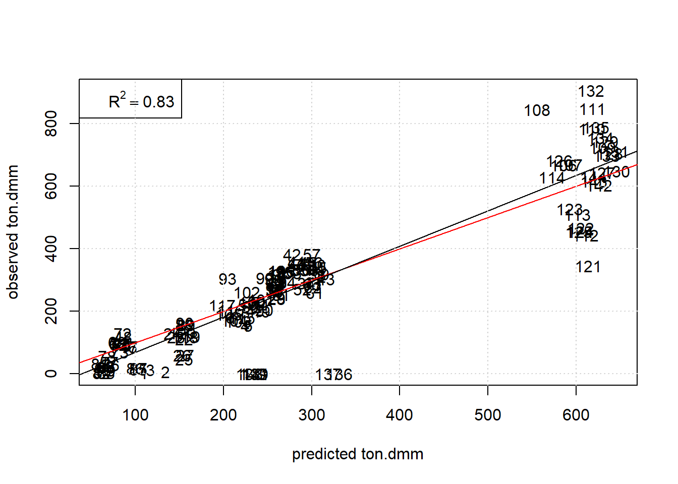
Figure 7.2: Plot observed ton.dmm versus Random Forest predictions with obs# as plot label. The red and black line denote the diagonal and regression line, respectively.
The Random Forest describes the data well within replication error except for a few outlying no-responders (note: the hyperparameter mtry has been validated by another script to be 2 based on 10-fold crossvalidation with consequtive blocks).
The next program chunk creates a 4-dimensional grid (m.kat x m.add x p.co2 x T) given t.h, p.h2 and v.ml at median values and plots it as 5-D Trellis plot, figure 7.2.
x.pred <- expand.grid(
    m.kat = seq(min(x.historical$m.kat,na.rm=T),
                max(x.historical$m.kat,na.rm=T), length=15),
    m.add = seq(min(x.historical$m.add),
                max(x.historical$m.add), length=15    ),
    p.co2 = seq(min(x.historical$p.co2),
                max(x.historical$p.co2), length=3    ),
    T     = seq(min(x.historical$T),
                max(x.historical$T), length=3  ),
    t.h   =median(x.historical$t.h),
    p.h2 =median(x.historical$p.h2),
    v.ml =median(x.historical$v.ml))
x.pred$y1 <- predict(rf.models[[1]],x.pred)
wireframe(y1 ~ m.kat*m.add|p.co2*T, data=x.pred,
                zlab=list(label="dmm",cex=0.7,rot=90),
                xlab=list(label="m.kat",cex=0.7,rot=0),
                ylab=list(label="m.add",cex=0.7,rot=0),
                drape=TRUE,
                at=do.breaks(c(50,600),100),
                col.regions = parula(100),
                strip=TRUE, pretty=TRUE,
                scales = list(arrows = FALSE,
                              x=c(cex=0.7),
                              y=c(cex=0.7),
                              z=c(cex=0.7)) ,
                screen = list(z = 300, x = -55, y=0)  ,
                par.strip.text=list(cex=1.2),
                layout=c(3,3),
                cuts=1000,
                par.settings = list(superpose.line = list(lwd=3))
  )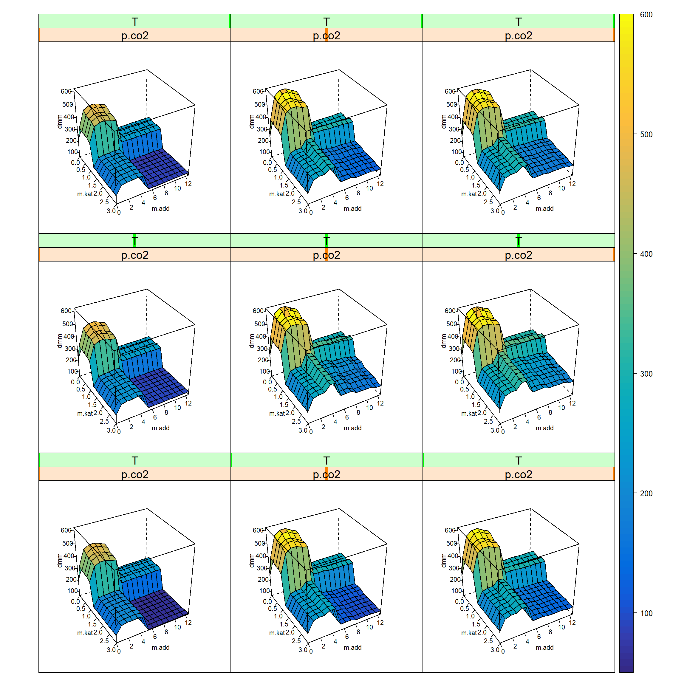
Figure 7.3: 5-D trellis plot ton.dmm=f(m.kat, m.add, p.co2, T) given t.h, p.h2, v.ml at median values. The outer x-axis is p.co2 and the outer y-axis refers to T.
The trellis-plot, figure 7.3, reveals four different domains of activity in the m.kat x m.add subspace. This suggests to select all trials with condition ton.dmm>400 as potential candidates for further optimization (step III in figure 7.1).
7.2 First augmentation (DoE1; step IV & V in figure 7.1)
The following code chunk selects nine high-performing candiate points from the historical record with the condition ton.dmm>400. In this subset T, p.h2, p.co2 and t.h were found constant at T=90, p.h2=90, p.co2=20 and t.h=18 thereby suggesting to conditionally optimize m.kat, v.ml and m.add first while keeping the remaining 4 variables constant at T=90, p.h2=90, p.co2=20 and t.h=18 for the time being.
A full factorial 33 grid design is created as a set of potential candidate points and the nine runs from above were augmented by another set of six runs optimally selected from the candidate set so as to render a full second order design of the factors m.kat, v.ml, m.add estimable (step III in figure 7.1).
library(AlgDesign)
# select promising subspace (9 unique runs)
# based on RF analysis and augment D-optimally
x.promising<- unique(x.historical[x.historical$ton.dmm>400,x.var])
dim(x.promising) # 9 x 7
## [1] 9 7sapply(x.promising,range) ## m.kat v.ml m.add T p.h2 p.co2 t.h
## [1,] 0.1875 0.25 0.78125 90 90 20 18
## [2,] 0.7500 0.50 3.12500 90 90 20 18# show ranges; note T, p.h2, p.co2, t.h being constant
# create full factorial candidate set 3 x 3 x 3
candidate <- expand.grid(
m.kat=seq(min(x.promising$m.kat),
max(x.promising$m.kat) ,length=3),
v.ml=seq(min(x.promising$v.ml),
max(x.promising$v.ml) ,length=3),
m.add=seq(min(x.promising$m.add),
max(x.promising$m.add) ,length=3) )
candidate <- rbind(x.promising[,1:3],candidate)
# rowbind x.promising and candidate set
set.seed(12345)
doe.cat <- optFederov(~ (m.kat + v.ml + m.add)^2+
I(m.kat^2) + I(v.ml^2) + I(m.add^2),
data=candidate,center=T,augment=T,rows=(1:9),
criterion="D", nTrials=15)$design
# d-optimal cat design
# comprising 9 historical
# and 6 additional candidates from candidate set
rownames(doe.cat ) <- NULL
## check condition number of augmeneted design,
# 1 indicates a perfectly hypersherical design,
# large positive number >>1 indicate poor designs
kappa(model.matrix(~ (m.kat + v.ml + m.add)^2 +
I(m.kat^2) + I(v.ml^2) + I(m.add^2) ,
data=data.frame(scale(doe.cat) ) ) )## [1] 8.519979doe.cat <- data.frame(obsnr=1:15,doe.cat)
knitr::kable(
doe.cat, booktabs = TRUE,row.names=F,align="c",
caption = 'D-optimal RSM design in (m.kat, v.ml, m.add)
comprising historical high responders
1-9 and D-optimal augmentation trials 10-15')| obsnr | m.kat | v.ml | m.add |
|---|---|---|---|
| 1 | 0.18750 | 0.500 | 0.781250 |
| 2 | 0.37500 | 0.500 | 1.562500 |
| 3 | 0.75000 | 0.500 | 3.125000 |
| 4 | 0.37500 | 0.500 | 0.937500 |
| 5 | 0.37500 | 0.500 | 1.250000 |
| 6 | 0.37500 | 0.500 | 1.875000 |
| 7 | 0.37500 | 0.500 | 2.187500 |
| 8 | 0.37500 | 0.500 | 2.500000 |
| 9 | 0.37500 | 0.250 | 1.562500 |
| 10 | 0.75000 | 0.250 | 0.781250 |
| 11 | 0.75000 | 0.500 | 0.781250 |
| 12 | 0.75000 | 0.375 | 1.953125 |
| 13 | 0.18750 | 0.250 | 3.125000 |
| 14 | 0.75000 | 0.250 | 3.125000 |
| 15 | 0.46875 | 0.375 | 3.125000 |
The augmentation trials #10-#15 were run in the laboratory (results for #1-#9 are already available) and DoE1 was analyzed with stepwise OLS.
7.3 Modeling DoE1 (step VI & VII in figure 7.1)
The analysis of well-designed experiments is relatively straightforward. Because the data has been designed with an underlying parametric model assumption (here: a full second order RSM design), all model terms are unconfounded (orthogonal) and can be easily estimated with stepwise OLS.
DoE1 is available in the Excel sheet “DoE1” and is of dimension 44x10. X-variables are at position# 2-4 Y-variables are at position 9-10
7.4 Analysis of DoE1
The code reads the data from DoE1, assigns X- and Y-variables, does the OLS modeling and reports R2 values of the fit.
library(MASS)
doe1 <- as.data.frame(read_excel(input,
               sheet="DoE1"))
dim(doe1)  # 44 x 10
## [1] 44 10x.var <- colnames(doe1)[2:4]
y.var <- colnames(doe1)[9:10]
ols.models <- list()
R2 <- NULL
form <- "~ (m.kat + v.ml + m.add)^2 + I(m.kat^2) +
I(v.ml^2) + I(m.add^2) "# parametric formula for
# linear model
for (i in (1:length(y.var)) ) {# step-OLS modeling;
# add models to list ols.models
ols.models[[i]] <- stepAIC(lm(formula(paste(y.var[i],form, sep="")),
data=doe1,x=T,y=T),trace=0,
k = log(nrow(doe1))) # BIC criterion
R2 <- c(R2, round(cor(predict(ols.models[[i]]),
doe1[,y.var[i]])^2,2))
}
names(R2) <- y.var
R2 # show fit in terms of R2## ton.dmm ton.mf
## 0.91 0.97Simple graphical model diagnostics, figure 7.4, here scatter plot observed values versus OLS-predictions, reveal an unbiased fit, with the model depicted as trellis plot in figure 7.5
plot(predict(ols.models[[1]]), doe1$ton.dmm,type="n",
     xlab="predicted ton.dmm", ylab="observed ton.dmm")
text(predict(ols.models[[1]]), doe1$ton.dmm,labels=doe1$obsnr)
abline(0,1,col="red")     # diagonal in red
abline(lm(doe1$ton.dmm~predict(ols.models[[1]]))$coef,lty=2)
legend("topleft",legend=substitute(R^2 == a, list(a=R2[1])   )   )
# linear fit in black
grid()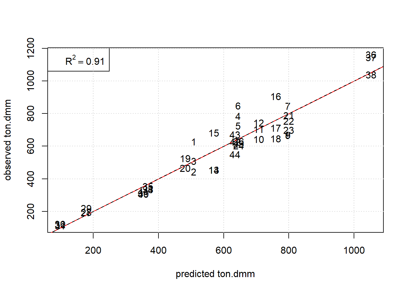
Figure 7.4: Observed ton.dmm versus OLS predictions of the RSM design with obs# being used as plot label. The red and black line denote the diagonal and regression line, respectively.
## show ton.dmm = g3(m.kat,m.add,v.ml) as trellis plot
x.pred <- expand.grid(m.kat = seq(min(doe1$m.kat),
                                  max(doe1$m.kat), length=15    ),
                      m.add = seq(min(doe1$m.add),
                                  max(doe1$m.add), length=15    ),
                      v.ml  = seq(min(doe1$v.ml),
                                  max(doe1$v.ml), length=3    )  )
x.pred$y1 <- predict(ols.models[[1]],x.pred)
wireframe(y1 ~ m.kat*m.add|v.ml, data=x.pred,
                zlab=list(label="dmm",cex=1.2,rot=90),
                xlab=list(label="m.kat",cex=1.2,rot=0),
                ylab=list(label="m.add",cex=1.2,rot=0),
                drape=TRUE,
                at=do.breaks(c(100,1200),100),
                col.regions = parula(100),
                strip=T,
                scales = list(arrows = FALSE,
                              x=c(cex=1.2),
                              y=c(cex=1.2),
                              z=list(cex=1.2) ),
                screen = list(z = 300, x = -60, y=0),
                par.strip.text=list(cex=1.2),
                layout=c(3,1)
)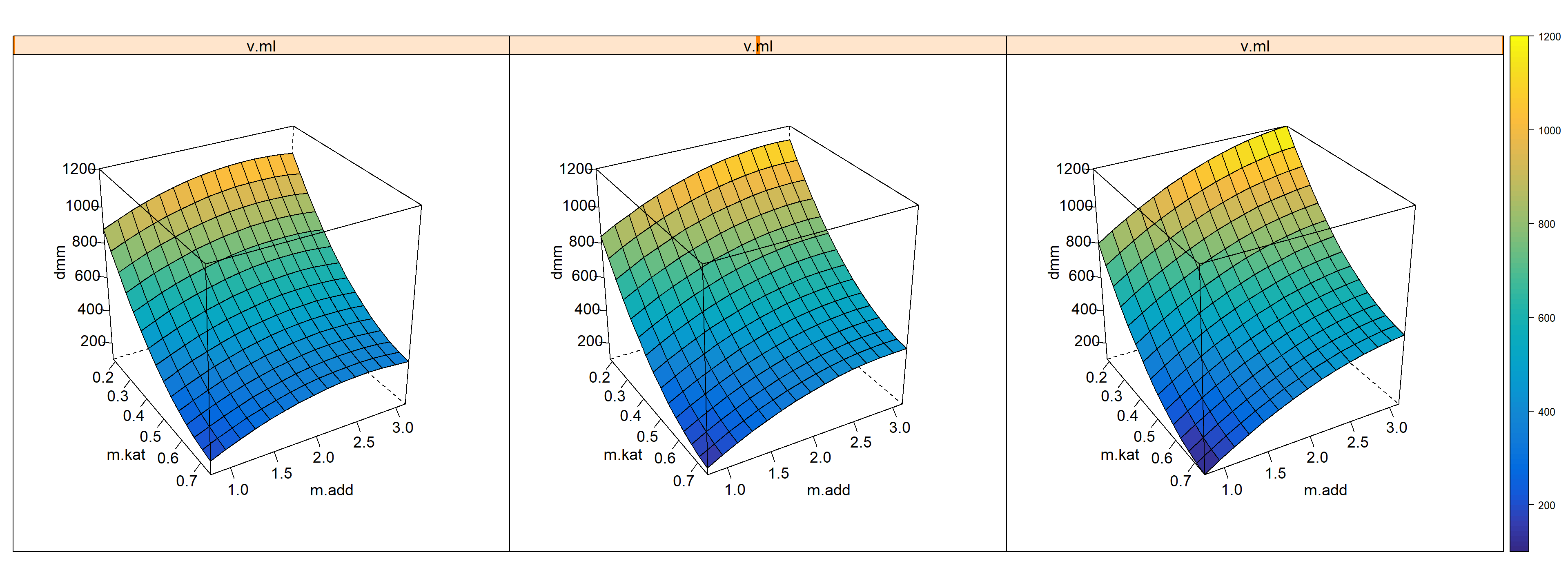
Figure 7.5: 4-D Trellisplot ton.dmm=f(m.kat,m.add,v.ml) given T=90, p.h2=90, p.co2=20 and t.h=18
7.5 Optimization and relaxation of DoE1 (step VIII in figure 7.1)
In the optimization step the above OLS model is maximized subject to box-constraints and the box-constraints are subsequently relaxed in discrete steps with stepsize 10, 20 and 30% of the initial space thereby creating a sequence of three relaxation trials to be realized in the laboratory.
The rationale of relaxation as an exploratory tool for making rapid progress was discussed in detail in chapter 6 and is again graphically sketched in figure 7.6.
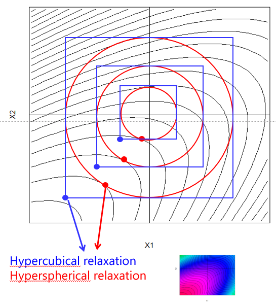
Figure 7.6: Two-dimensional example of hypercubical and hyperspherical relaxation
With \(\Delta X\) being the stepsize of the relaxation, in the code chunk taken to be 10% of the initial design space, that is \(\Delta X = 0.1 \cdot (UB - LB)\), and LB and UB denoting the lower and upper bounds of the process factors, respectively, the optimization and relaxation problem can be stated as follows
\[\max_{X} f(X)\] subject to hypercubical constraints: \[(LB - k \cdot\Delta X) \leq X \leq (UB + k \cdot\Delta X)\]
or alternatively subject to hyperspherical constraints: \[\sum_{i=1}^Ix^2_{i} \leq (R + k \cdot\Delta r)^2\] with R denoting the radius to be relaxed with stepsize \(\Delta r\).
By varying k=1,2,3… and running the optimization, a sequence of relaxation trials is generated in the direction of steepest ascend of ton.dmm to be realized in laboratory.
Note that in the present code hypercubical rather than hypersperical constraints are being applied.
library(Rsolnp)
x.var          <- colnames(doe1)[2:4]
x.mean         <- sapply(doe1[,x.var],mean,na.rm=T)
names(x.mean)  <- x.var
x.lb           <-  sapply(doe1[,x.var],min,na.rm=T)
x.ub           <-  sapply(doe1[,x.var],max,na.rm=T)
delta          <- (x.ub-x.lb)/10 # stepsize 10% of initial design

df.collect  <- NULL

#########################
# given predictors x the function returns
# OLS predictions y=g(x) for each
y.val   = function(x) {
  xx               <- data.frame(rbind(x))
  colnames(xx)     <- x.var
  collect          <- NULL
  for (iii in (1:length(y.var)) )   {
    collect <- c(collect,predict(ols.models[[iii]],xx))
  }
  return( collect  )
}

objective   =function(x) {
  xx               <- data.frame(rbind(x))
  colnames(xx)     <- x.var
  return( -predict(ols.models[[1]],xx)  )#note: -obj <=> max(obj)
}
###
for (i in (1:3))   {

  xx.lb <- x.lb - i*delta
  xx.ub <- x.ub + i*delta

  tt <- system.time(res  <- solnp(fun=objective,
                            pars=x.mean,
                            LB=xx.lb,UB=xx.ub,
                            control=list(trace=0)))

  x.solution         <- res$pars
  y.opt              <- y.val(x.solution)
  names(y.opt)       <- y.var


  df.collect  <- rbind(df.collect,
                       data.frame(relax.step=i*10,
                       target="max(ton.dmm)",
                       rbind(x.solution),rbind(y.opt),
                       stringsAsFactors =FALSE,
                       t.min=round(tt[3]/60,2) )  )

}
rownames(df.collect)  <- NULL

df.collect
## relax.step target m.kat v.ml m.add ton.dmm ton.mf t.min
## 1 10 max(ton.dmm) 0.13125 0.5249999 3.359373 1363.439 1080.125 0
## 2 20 max(ton.dmm) 0.07500 0.5499999 3.575959 1529.786 1303.163 0
## 3 30 max(ton.dmm) 0.01875 0.5749999 3.659436 1707.569 1544.425 0| relax.step | target | m.kat | v.ml | m.add | ton.dmm | ton.mf | t.min |
|---|---|---|---|---|---|---|---|
| 10 | max(ton.dmm) | 0.13 | 0.52 | 3.36 | 1363.44 | 1080.13 | 0 |
| 20 | max(ton.dmm) | 0.08 | 0.55 | 3.58 | 1529.79 | 1303.16 | 0 |
| 30 | max(ton.dmm) | 0.02 | 0.57 | 3.66 | 1707.57 | 1544.42 | 0 |
The reported response values for ton.dmm and ton.mf in the result table 7.3 from relaxation are model predictions and not measured values.
In the laboratory the following results, table 7.4, were experimentally realized
| Relaxation% | m.kat | v.ml | m.add | ton.dmm | ton.mf |
|---|---|---|---|---|---|
| 10 | 0.13 | 0.52 | 3.36 | 1373.56 | 1559.56 |
| 20 | 0.08 | 0.55 | 3.58 | 1374.59 | 2761.87 |
| 30 | 0.02 | 0.57 | 3.66 | 179.56 | 1039.71 |
Based on these results, table 7.4, the second trial was selected as a candidate for further optimization. Note the sharp drop of the third relaxation trial (30%) compared to the model predictions. This likely indicates that a local maximum was exceeded in the course of the relaxation.
Given this finding m.kat, v.ml and m.add are considered locally optimal (hereafter referred to as m.kat#, v.ml#, m.add#) and further optimization will focus on the factors T, p.h2, p.co2, t.h so far kept constant.
7.6 Linear DoE2 (step IX & V in figure 7.1)
A small linear saturated design was created comprising five unique runs in the parameters T, p.h2, p.co2, t.h given m.kat#, v.ml# and m.add#.
library(AlgDesign)
## full factorial candidate set
candidate <- expand.grid(T=seq(80,  100 ,length=2),
                         p.H2=seq(80,  100 ,length=2),
                         p.CO2=seq(15,  25 ,length=2),
                         t.H=seq(16,  20 ,length=2) )
set.seed(12345)
doe2 <- optFederov(~ T + p.H2 + p.CO2 + t.H ,
                      data=candidate,center=T,
                      criterion="D", nTrials=5)$design
# d-optimal cat design
(kappa <- kappa(model.matrix(~ T + p.H2 + p.CO2 + t.H ,
                   data=data.frame(scale(doe2)   )   ) ))
## [1] 1.499816# 1.499816
rownames(doe2) <- NULL
doe2 <- data.frame(obsnr=1:5,doe2)
knitr::kable(
doe2, booktabs = TRUE,row.names=F,digits=2,format="pandoc",
caption = 'Linear D-optimal design with
20% relaxation trial from table 7.4 as centerpoint')| obsnr | T | p.H2 | p.CO2 | t.H |
|---|---|---|---|---|
| 1 | 80 | 80 | 15 | 16 |
| 2 | 100 | 100 | 25 | 16 |
| 3 | 100 | 100 | 15 | 20 |
| 4 | 100 | 80 | 25 | 20 |
| 5 | 80 | 100 | 25 | 20 |
Note that the design is next to orthogonal with \(\kappa\)=1.5!
Analysis and relaxation of DoE2 is similar to the steps already described.
7.7 Analysis of DoE2 (step VI & VII in figure 7.1)
doe2 <- as.data.frame(read_excel(input,
                  sheet="DoE2"))
dim(doe2)  # 21 x 10
## [1] 21 10x.var <- colnames(doe2)[5:8]
y.var <- colnames(doe2)[9:10]
ols2.models <- list()
R2 <- NULL
form <- "~ T + p.h2 + p.co2 + t.h "
# parametric formula for linear
# models in R notation
for (i in (1:length(y.var)) ) { # add OLS models to list ols2.models
ols2.models[[i]] <- stepAIC(lm(formula(paste(y.var[i],form, sep="")),
data=doe2,x=T,y=T),trace=0,
k = log(nrow(doe2)))
R2 <- c(R2, round(cor(predict(ols2.models[[i]]),
doe2[,y.var[i]])^2,2))
}
names(R2) <- y.var
R2 # show fit in terms of R2## ton.dmm ton.mf
## 0.92 0.78# show fit as plot observed versus predicted (only ton.dmm showns)
plot(predict(ols2.models[[1]]), doe2$ton.dmm,
type="n",xlab="predicted ton.dmm", ylab="observed ton.dmm")
text(predict(ols2.models[[1]]), doe2$ton.dmm,labels=doe2$obsnr)
abline(0,1,col="red") # diagonal in red
abline(lm(doe2$ton.dmm~predict(ols2.models[[1]]))$coef,lty=2)
# linear fit in black
grid()
legend("topleft",legend=substitute(R^2 == a, list(a=R2[1]) ) )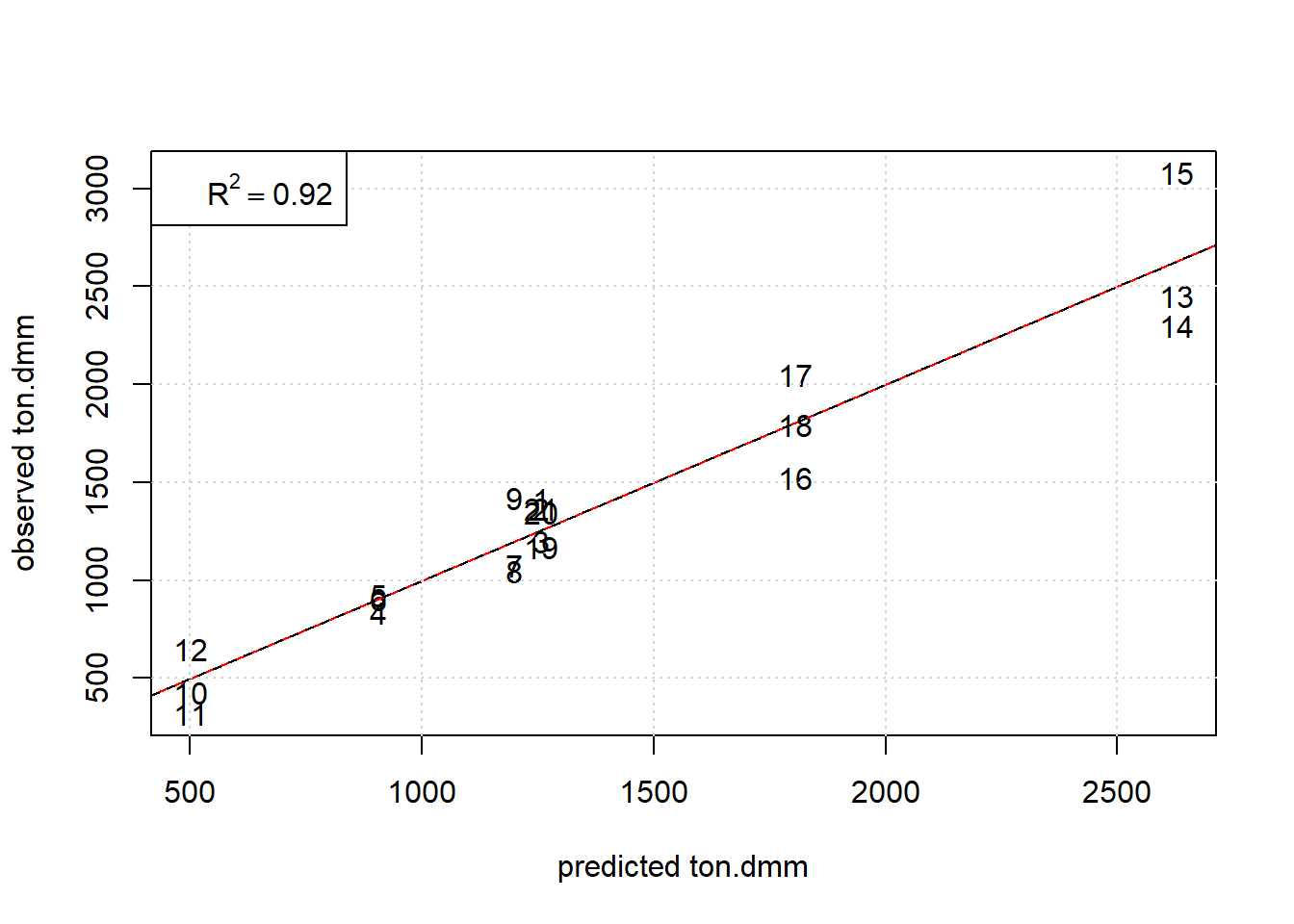
Figure 7.7: Observed ton.dmm versus OLS predictions ton.dmm=f(T, p.h2, p.co2,t.h) given m.kat=0.075, v.ml=0.55, m.add=3.576. The red and black line denote the diagonal and regression line, respectively.
###### trellis plot of OLS2 effectsx.pred <- expand.grid( T = seq(min(doe2$T),
max(doe2$T), length=15),
p.h2 = seq(min(doe2$p.h2),
max(doe2$p.h2), length=15 ),
p.co2 = seq(min(doe2$p.co2),
max(doe2$p.co2), length=3),
t.h = seq(min(doe2$t.h),
max(doe2$t.h), length=3))
x.pred$y1 <- predict(ols2.models[[1]],x.pred)
wireframe(y1 ~ T*p.h2|p.co2*t.h, data=x.pred,
zlab=list(label="dmm",cex=1,rot=90),
xlab=list(label="T",cex=1,rot=0),
ylab=list(label="p.h2",cex=1,rot=0),
drape=TRUE,
at=do.breaks(c(-50,2600),100),
col.regions = parula(100),
strip=T,
scales = list(arrows = FALSE,
x=c(cex=1),
y=c(cex=1),
z=c(cex=1)) ,
screen = list(z = 60, x = -55, y=0), layout=c(3,3) ,
par.strip.text=list(cex=1.2) )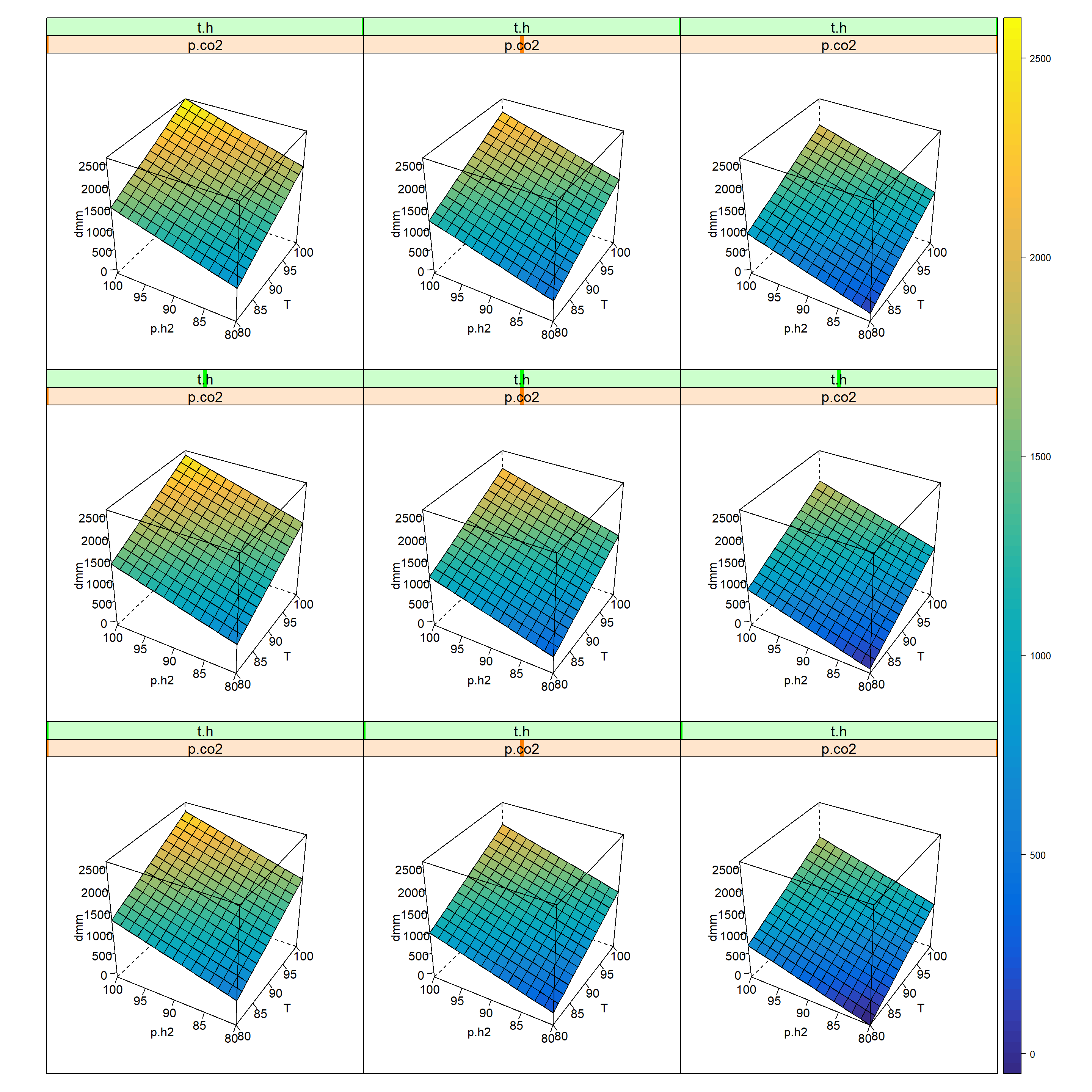
Figure 7.8: 5-D Trellis plot of ton.dmm=f(T, p.h2, p.co2, t.h) given m.kat=0.075, v.ml=0.55, m.add=3.576
7.8 Optimization and relaxation of DoE2 (step VIII in figure 7.1)
x.var          <- colnames(doe2)[5:8]
x.mean         <- sapply(doe2[,x.var],mean,na.rm=T)
names(x.mean)  <- x.var
x.lb           <-  sapply(doe2[,x.var],min,na.rm=T)
x.ub           <-  sapply(doe2[,x.var],max,na.rm=T)
delta          <- (x.ub-x.lb)/4
# stepsize 25% of initial design

df.collect  <- NULL

#########################
# given predictors x the function returns
# OLS predictions y.j=g.j(x) for each y.j
y.val   = function(x) {
  xx               <- data.frame(rbind(x))
  colnames(xx)     <- x.var
  collect          <- NULL
  for (iii in (1:length(y.var)) )   {
    collect <- c(collect,predict(ols2.models[[iii]],xx))
  }
  return( collect  )
}
objective   =function(x) {
  xx               <- data.frame(rbind(x))
  colnames(xx)     <- x.var
  return( -predict(ols2.models[[1]],xx)  )
  # note: -obj <=> max(obj)
}
###
for (i in (0:2))   {

  xx.lb <- x.lb - i*delta
  xx.ub <- x.ub + i*delta
  tt <- system.time(res  <- solnp(fun=objective, pars=x.mean,
                            LB=xx.lb,UB=xx.ub,
                            control=list(trace=0)))

  x.solution    <- res$pars
  y.opt         <- y.val(x.solution)
  names(y.opt)  <- y.var
  df.collect    <- rbind(df.collect, data.frame(relax.step=i*25,
                        target="max(ton.dmm)",rbind(x.solution),
                        rbind(y.opt), stringsAsFactors =FALSE,
                        t.min=round(tt[3]/60,2) )  )

}
rownames(df.collect)  <- NULL
df.collect
## relax.step target T p.h2 p.co2 t.h ton.dmm ton.mf t.min
## 1 0 max(ton.dmm) 100 100 15.0 20 2627.845 2407.657 0
## 2 25 max(ton.dmm) 105 105 12.5 21 3313.269 2262.819 0
## 3 50 max(ton.dmm) 110 110 10.0 22 3998.693 2117.981 0| relax.step | target | T | p.h2 | p.co2 | t.h | ton.dmm | ton.mf | t.min |
|---|---|---|---|---|---|---|---|---|
| 0 | max(ton.dmm) | 100 | 100 | 15.0 | 20 | 2627.85 | 2407.66 | 0 |
| 25 | max(ton.dmm) | 105 | 105 | 12.5 | 21 | 3313.27 | 2262.82 | 0 |
| 50 | max(ton.dmm) | 110 | 110 | 10.0 | 22 | 3998.69 | 2117.98 | 0 |
The following table shows the experimental results of the above relaxation trials achieved in the lab, reported as mean values of triple replicates.
| Relaxation | T | p.h2 | p.co2 | t.h | ton.dmm | ton.mf |
|---|---|---|---|---|---|---|
| 0 | 100 | 100 | 15.0 | 20 | 2563.43 | 2401.47 |
| 25 | 105 | 105 | 12.5 | 21 | 2760.86 | 1768.81 |
| 50 | 110 | 110 | 10.0 | 22 | 2208.56 | 1275.56 |
Again, the second relaxation trial (25%) shows a small improvement which turns out reproducible upon replication, while the third relaxation candidate (50%) performs comparatively poor in both responses.
7.9 Conclusion
Figure 7.9 is a graphical summary of the achieved improvement of ton.dmm and ton.mf, both in terms of location (mean values) and dispersion (standard deviation).
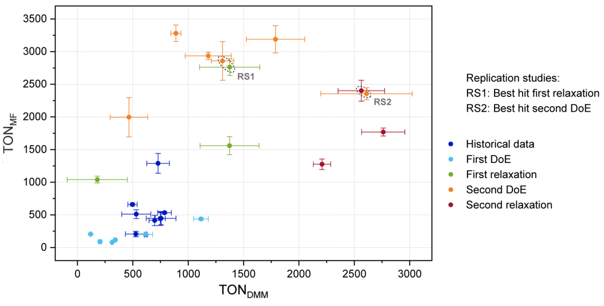
Figure 7.9: Summary of improvements over all optimization steps. The error bars denote one standard deviation based on three replicates
Comparison of the raw figures of the optimization project is impressive: With 46 unique trials in the historical record a ton.dmm lift of \(3.9 \rightarrow 786\) was achieved which boils down to \(lift/trial \approx 17\).
In the present algorithmically driven workflow, a \(lift/trial \approx 165\) was achieved in 16 DoE1,2 and relaxation trials that revealed a lift \(119 \rightarrow 2761\). Based on these figures multivariate methods are found to be approximately ten-times more effective than one-factor-at-the-time optimization.
Reference
Siebert M., Krennrich G., Seibicke M., Siegle A.F., Trapp O. 2019. “Identifying High-Performance Catalytic Conditions for Carbon Dioxide Reduction to Dimethoxymethane by Multivariate Modelling.” Chemical Science 10:45. https://pubs.rsc.org/en/content/articlelanding/2019/sc/c9sc04591k#!divAbstract.
T. Hastie, R. Tibshirani, J. Friedman. 2009. The Elements of Statistical Learning. 2nd ed. Springer-Verlag.