3 Two introductory examples

Before discussing the statistical details of linear models, a model class with very wide use in the statistical sciences and the major tool of DoE, a few thoughts about the classical one-factor-at-the-time (OFAT) optimization are appropriate, as they can help introducing some concepts of statistical model building and optimization.

3.1 Example I: Optimization in one dimension

In this chapter a simple one-dimensional example will be used to introduce some helpful statistical concepts, namely

1. What is a statistical model?
2. Pure Error (PE) versus model bias (Lack of Fit, LoF)
3. Inter- and extrapolating statistical models and identifying directions of ascent/descent

Imagine a one-dimensional optimization project with the objective of finding the concentration, \(conc^*\), maximizing yield=f(conc). Design space (factor range), budget (number of experiements) and design (DoE) are given as follows

1. Chemically sensible range for conc
   • 1 - 3 mmol/l
2. Research budget
   • 9 runs
3. DoE1
   • spread runs equidistantly across range and measure yield at the nine concentration values

The results from runnning the equidistant one-factor design, DoE1, are listed in table 3.1 and depicted in figure 3.1 as simple yield~conc scatter plots with four different models (interpretations) superimposed.

Table 3.1: Results of one-dimensional optimization of yield over concentration, DoE1; Max[yield=f(conc)]

Obsnr	conc	yield
1	1.00	46.39
2	1.25	46.13
3	1.50	58.13
4	1.75	63.09
5	2.00	65.49
6	2.25	62.30
7	2.50	69.57
8	2.75	70.13
9	3.00	67.09

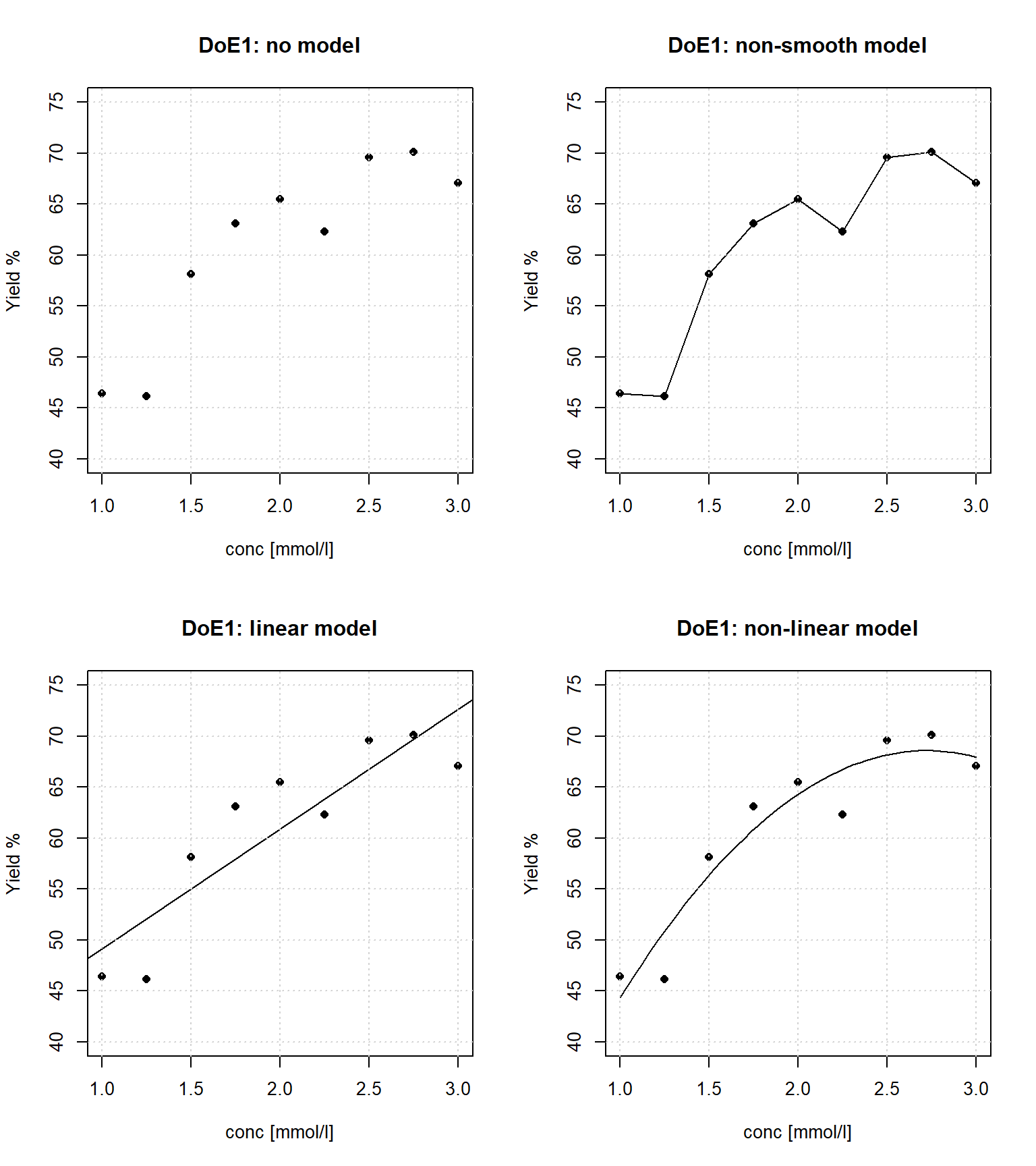
Figure 3.1: Different models (interpretations) of the data from table 3.1; DoE1

Figure 3.1 interprets the raw data in four different way

1. No model
   • data is plotted “as is” without making any model assumption.
2. Non-smooth “model”
   • This model consists of a solid line connecting data points and helps the observer in recognizing patterns such as trends, minima and maxima. It ignores experimental uncertainty by assuming the measurements to be exact and and free from errors. The slope of the connecting line (the gradient) changes at each support point in a steplike manner, a behaviour unlikely to be found in nature⁷.
3. Linear model
   • The data is being interpolated with a straight line so as to fit the data in a least square sense. Mathematically, the model line is represented by a linear equation, \(yield = a_{0} + a_{1}\cdot conc\) with intercept and slope parameter \(a_{0}\) and \(a_{1}\), respectively.
4. Non-linear model
   • Here the data is being interpolated with a second order polynomial to account for non-linear effects, parametrically represented by the equation \(yield = a_{0} + a_{1}\cdot conc + a_{2}\cdot conc^2\)

The regression models, #3 and #4, are clearly advantageous when it comes to interpolating, extrapolating and optimizing the models and can be used to identify directions of ascend/descend. The model property of revealing gradients information is even more important in higher dimensions as the number of directions in \(\mathbb{R}^k\) grows exponentially (\(\approx 2^k\)). Finally, these smooth models account for experimental uncertainties (errors) as a natural part of the least squares fitting process as will be described later in more detail.

However, figure 3.1 reveals some weaknesses of the “equidistant” design when it comes to discriminating between model #4 and model #3, i.e. deciding which model suits the data best given experimental uncertainty. While model #4 indicates non-linear saturation or a maximum in the concentration range [2-3 mmol/l], model #3 suggests a linear increase beyond the upper bound⁸. The difficulty in distinguishing #3 from #4 lies in the design, DoE1, which makes it hard to differentiate between model bias and pure error.
Table 3.2, shows an alternative design, DoE2, generated by the above model and consisting of three triple replicates at three different concentration values conc={1,2,3}. DoE2 is depicted in figure 3.2 as scatter plots with linear and a non-linear models superimposed.

Table 3.2: Results of one-dimensional optimization of yield over concentration, \(\max_{conc} yield=f(conc)\), with an alternative design DoE2 consisting of three equidistant triple replicates in the concentration range [1-3 mmol/l]

obsnr	conc	yield
1	1	46.39
2	1	46.21
3	1	47.07
4	2	59.25
5	2	65.49
6	2	68.25
7	3	65.63
8	3	60.43
9	3	67.09

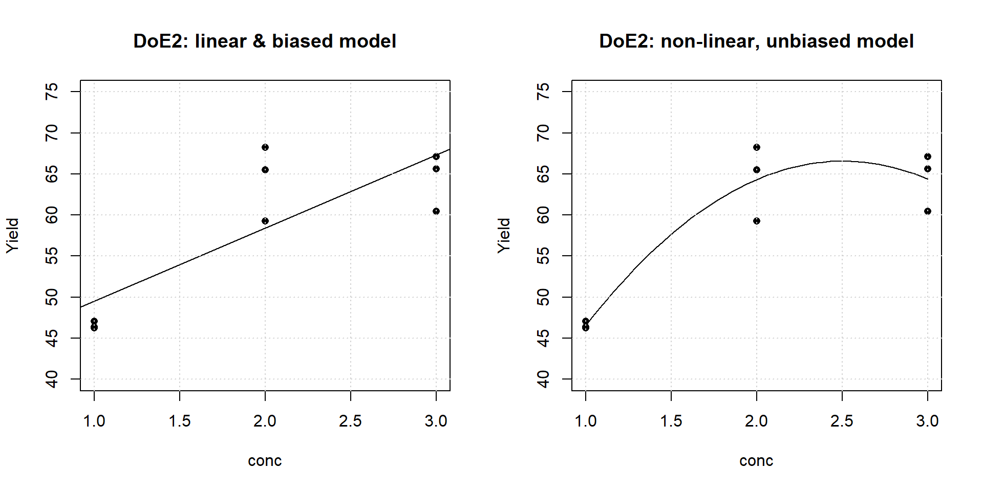
Figure 3.2: Linear biased and non-linear unbiased models of the design DoE2

DoE2 renders the task of discriminating between model #3 and model #4 easier: Figure 3.2 suggests the linear model to be biased, because the triple replicates at the center are not approriately described, whereas the non-linear model describes the data appropriately in the experimental concentration range, thereby supporting the saturation hypothesis from above. With \(\hat{y}\) denoting the model predictions and \(\bar{y}\) the mean average of the replicate triple, the model bias (=systematic error, Lack of Fit) is defined as the sum of squares (SS) \(SS_{\textrm{LoF}} = (\hat{y}-\bar{y})^2\) while the Pure Error (statistical error, PE) is given by \(SS_{\textrm{PE}} =\sum_{i}(y_{i}-\bar{y})^2\).

Figure 3.3 gives a graphical overview of the statistical elements that differentiates Lack of Fit from Pure Error.

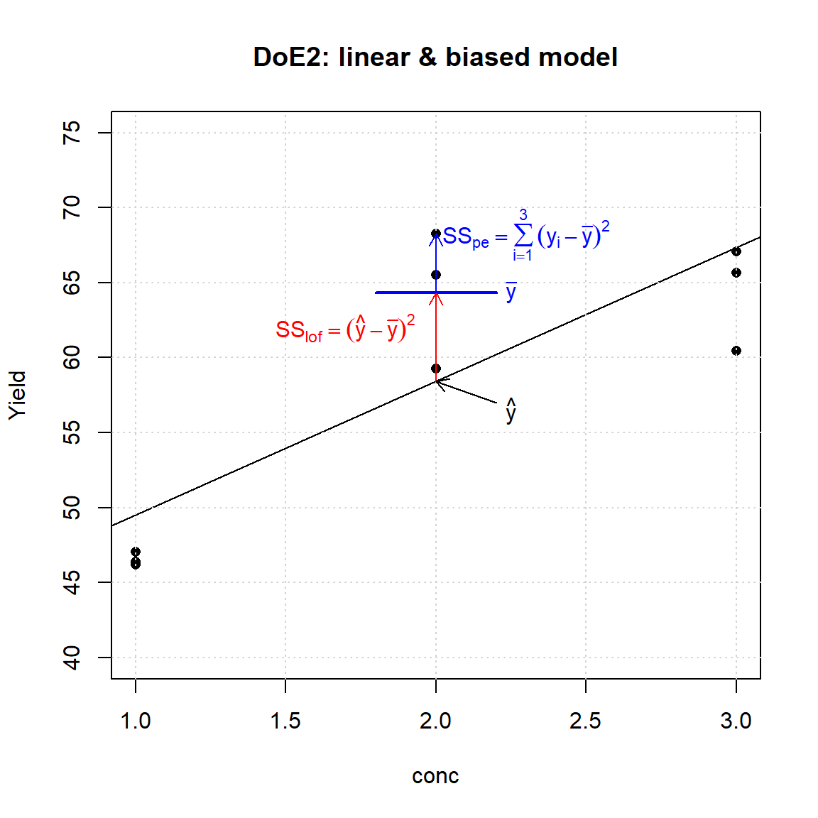
Figure 3.3: Lack of Fit (LoF, model bias) and Pure Error (PE)

3.2 Controlling nuisance parameters

There is a proverbial joke among statisticians about the relationship between the population size and storck numbers, allegedly observed in the German town Oldenburg between 1930-1936 (Ornithologische Monatsberichte, 44, Nr. 2 (1936), 48, Nr. 1 (1940), Berlin). The raw figures of this groundbreaking work are plotted in Figure 3.4 and reveal a strong and significant relationship between population and number of storcks.

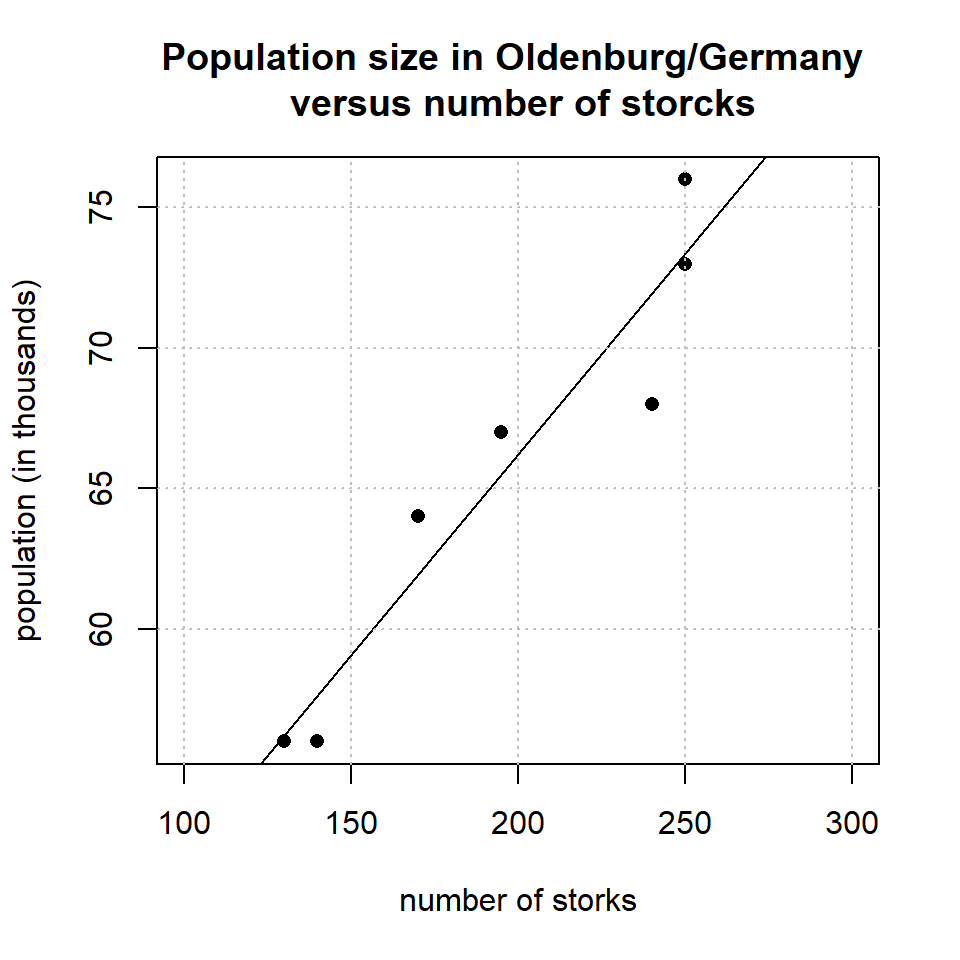
Figure 3.4: Population size in Oldenburg/Germany versus observed number of storcks

Now the question arises whether figure 3.4 is in support of the hypothesis that the storcks are bringing the babies and thereby affecting the size of the population? The correlation in figure 3.4 is much too strong to be dismissed as a chance result, and so there must be a hidden confounder explaining the strong relationship. Indeed, this confounder is easily identified to be the time as figure 3.5 illustrates.

Figure 3.5: Number of storcks and population size plotted versus time in Oldenburg/Germany between 1930-1936

As figure 3.5 shows, human and storck population share a common trend in time and that, by transitivity, shows up as a strong correlation between both variables \[Birth \leftrightarrow time \leftrightarrow Storck \] \[ \Rightarrow Birth \leftrightarrow Storck\] Whenever two variables share a common trend in time, they will be correlated nescessarily. This property makes time⁹ to the most dangerous confounder in the experimental sciences, and statisticians thought about ways and means to control this confounder. Fortunately, randomization is an effective way to eliminate potential bias from serial effects.
Controlling time effects by randomization is best understood with a simple one-dimensional example: A researcher wants to investigates the effect of temperature on the yield of a chemical reaction and sets up a simple One-Factor-at-the-Time (OFAT) design consisting of the six trials listed in table 3.3.

Table 3.3: OFAT optimization of yield over temperature, \(\max_{temp} [yield=f(temp)]\), without randomization of the design

run.order	temp	yield
1	100	56.4
2	105	62.8
3	110	67.3
4	115	59.0
5	120	69.3
6	125	71.5

“Eye-ball regression” of table 3.3 suggest a positive effect of temperature on yield. Unfortunately, this is not the only possible reading of the experimental results, and the outcome can be alternatively attributed to the positive effect of the run.order (or, here, time) on yield. Even worse, any linear combination of time and temperature, \(a_{1} \cdot \textrm{temp} + a_{2} \cdot \textrm{run.order} ; \ a_{1}, a_{2} \in \mathbb R\), is a valid reading of the outcome: The increase can be exclusively explained by time and temperature, however, any other “effect mixture” is similarily valid, and no statistical method can identify the individual coefficients \(a_{1}, a_{2}\). In the design, table 3.3, time and temperature are perfectly confounded (\(r_{temp ,time}=+1\)¹⁰), and thereby the individual effects become hidden. Confounding run.order and temp must be and can be avoided by “decorrelating” time and temperature by randomizing the experimental design as shown in table 3.4.

Table 3.4: OFAT optimization yield over temperature, \(\max_{temp} [yield=f(temp)]\), with randomization of the design

run.order	temp	yield
1	125	71.5
2	100	56.4
3	120	69.3
4	110	67.3
5	115	59.0
6	105	62.8

Randomization decorrelates time and temperature (\(r_{temp,time} = -0.37\)) and the regression model \(yield = b_{0} + b_{1} \cdot temp + b_{2} \cdot time\) can now be jointly identified as \(yield = 10.7(\pm 30.2) - 0.18(\pm1.25)\cdot time + 0.48(\pm 0.25) \cdot temp\). Randomization thus becomes an important instrument in DoE for controlling the influence of “confounders in time” and should be applied whenever possible. Usually, experimenters do not like randomization, as the logistics of the experimental program become more complex. However, the value of randomization exceeds by far the additional amount of logistics incurred. In chemistry, hidden time effects, such as temporal loss of catalytic activity or deterioration of analytical instruments over time, are realities not to be ignored. Nevertheless, there are situations where randomization cannot be applied such as running DoE on large scale plants¹¹. The consequence of lacking randomization will be, that all effects will be temporally biased, provided, of course, that serial effects are present.

3.3 Example II: Optimization in two dimensions

Section 3.1 and 3.2 introduced some helpful statistical concepts in the process of statistical model buiding with a one-dimensional example.
In the present section (3.3) the one dimensional example from section 3.1 will be augmented by another dimension for discussing the shortcomings of the one-factor-at-the-time method (OFAT) in higher dimensions. The problem is stated as an optimization problem, namely finding optimal reaction conditions \(conc^*\) and \(temp^*\) maximizing yield.
Sensible and feasible factor ranges are given as follows

1. conc: {76 - 104 mmol/l}
2. temp: {138 - 152 ⁰C}

Faced with such a problem, many researchers, not being familiar with multivariate methods, would intuitively turn to OFAT optimization by varying one variable first while keeping the other factor(s) constant.

In the present example, the researcher decided to start the OFAT process by keeping the temperature constant at temp=142[ ⁰C] and varying the concentration at four different levels. This OFAT design is shown in table 3.5 and depicted in figure 3.6.

Table 3.5: OFAT: vary conc|temp=142

temp	conc	yield
142	76	77.5
142	85	80.9
142	94	81.4
142	104	78.6

Figure 3.6: Conditional OFAT optimization \(\max_{conc} [yield=f(conc|temp=142)]\). The red line indicates the location of the OFAT maximum

Figure 3.6 suggests a conditional yield optimum at \(conc^*|(temp=142 [^0C^])) \approx 91 [mmol/l];\) \(yield^* \approx 82 [\%]\).
The next optimization round varies the temperature given the conditional OFAT optimum \(conc^*\approx 91 \ [mmol/l]\) as shown in table 3.6 and figure 3.7.

Table 3.6: OFAT: vary temp|conc=91

temp	conc	yield
138	91	76.0
142	91	81.6
148	91	85.4
152	91	84.8

Figure 3.7: Conditional OFAT optimization \(\max_{temp} [yield=f(temp|conc^*=91)]\). The red line indicates the location of the OFAT maximum

Figure 3.7 reveals a maximum at \(temp^* \approx 149 [^0C]\) with an expected yield, \(yield^* \approx 86 [\%]\). At this stage the OFAT optimization process stops and reports the OFAT maximum \[\boxed{conc^*=91[mmol/l];\ temp^*=149[^0C];\ yield^* \approx 86[\%]}\]

OFAT optimization is clearly a suboptimal optimization strategy as can be seen in figure 3.8 that shows the response surface of the model \(y=f(conc,temp)\) together with the overlayed OFAT optimization trials from tables 3.5 and 3.6. The “true” maximum within experimental space is found at the upper and lower bound of temp and conc, i.e. the true local optimum is \[\boxed{conc^*=76[mmol/l];\ temp^*=152[^0C];\ yield^* \approx 91[\%]}\] OFAT actually slices the experimental space thereby ignoring (because of not knowing) the local topology of the response surface. The local topology (response surface) depicted in figure 3.8 was obtained with a multivariate experimental design in the given factor ranges and suggests to increase the temperature and to decrease the concentration so as to further increase the yield beyond 91%.

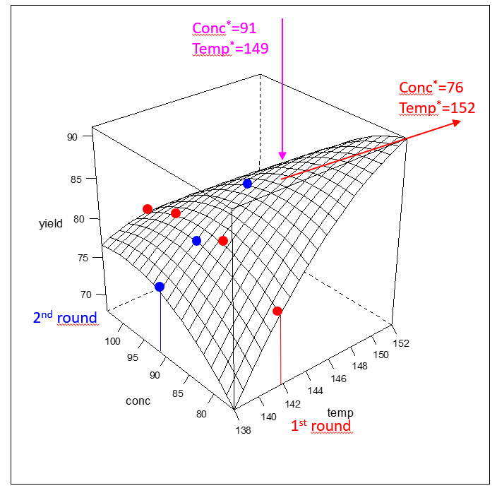
Figure 3.8: OFAT optimization seen from a multivariate perspective. The OFAT optimum is labelled magenta. OFAT trials are printed as blue and red dots. The direction of steepest ascent is indicated by the red arrow with the mutivariate optimum labelled red at the upper right corner of the design space

In high-dimensional space the OFAT optimization method gets even more laborious, cumbersome and ambigious. Given a set of process factors \(x_{1},x_{2},x_{3},....x_{I}\), the univariate OFAT process starts by ambiguously selecting one variable to be varied while keeping the other factors constant at specific values, formally \[\Delta x_{i}|x_{j\neq i}=\textrm{const}_{j}\] and then works its way throught the whole set of variables \(x_{1},x_{2},x_{3},....x_{I}\). This process is tedious and error prone and will almost certaintly miss local optima with higher performance in high-dimensional space.

3.4 An introduction into linear statistical model building

In this chapter the basic principles of linear least squares models will be introduced, one of the most versatile statistical modeling class. Linear models have wide use in the empirical sciences and can be used for predictions, inference and optimization.

3.4.1 The elements of statistical inference

Statistical inference is, shortly stated, the method for making rational decisions in the presence of uncertainty and is an integral part of empirical model building and a prerequisite for understanding linear models. Fortunately, understanding one statistical test is sufficient for understanding all statistical tests, and there are many, as the logic of statistical testing turns out to be the same for all tests.
As a start let us consider the normal distribution with its probability density function (pdf) given by the analytic expression (3.1)¹²

\[\begin{equation} pdf(x\mid \mu ,\sigma ^{2})={\frac {1}{\sqrt {2\pi \sigma ^{2}}}}e^{-{\frac {(x-\mu )^{2}}{2\sigma ^{2}}}} \tag{3.1} \end{equation}\]

The normal distribution has two free parameters:

1. The location parameter \(\mu\) which determines the location of the maximum of the pdf.
2. The dispersion parameter \(\sigma\) which determines the spread (width) of the distribution.

The normal distribution, equation (3.1), can be abbreviated by \(N(\mu,\sigma)\). Two examples of this well-known, bell-shaped distribution are depicted in figure 3.9.

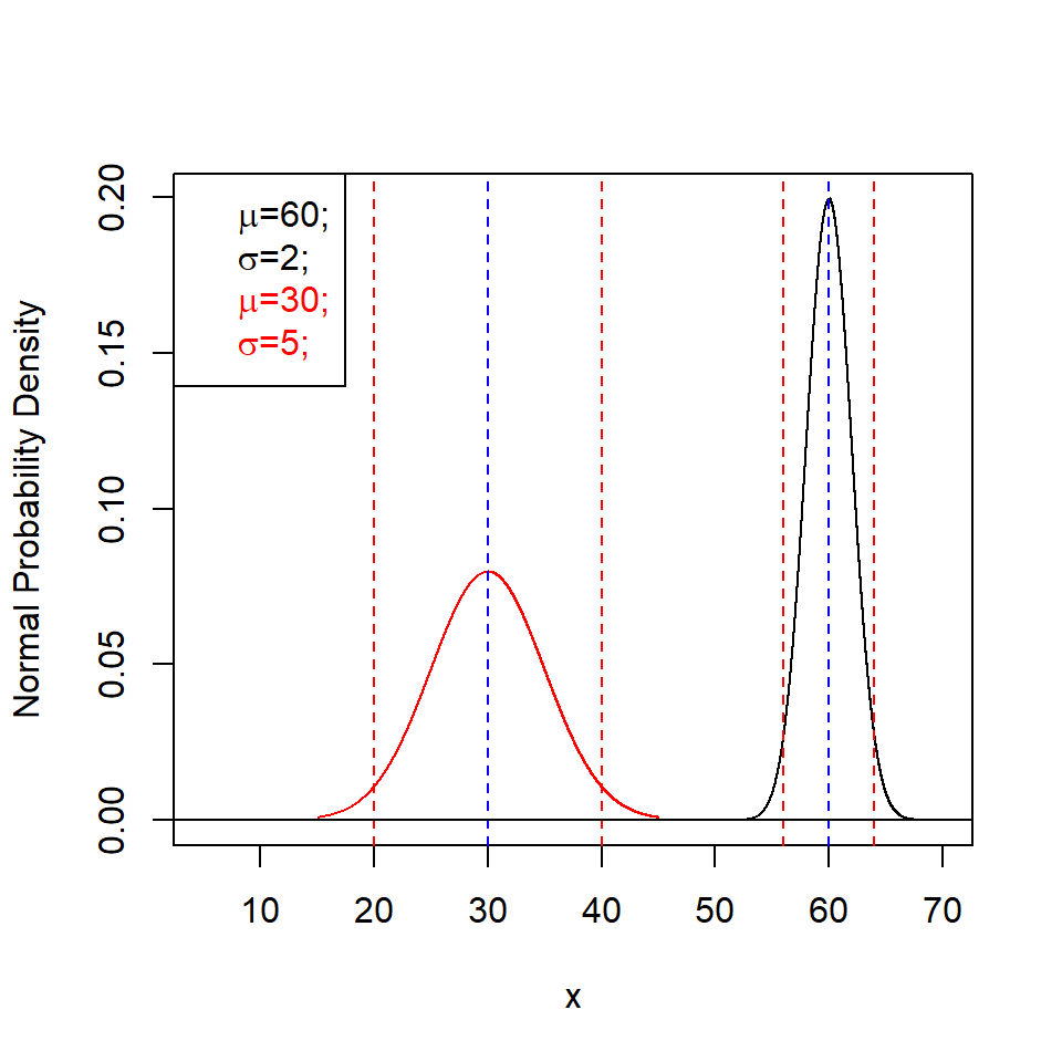
Figure 3.9: Normal probability density with two different location (blue) and dispersion parameters; \(\pm 2 \sigma\) limits are labelled red

Finite samples of size N from the normal distribution \(N(\mu,\sigma^2)\) can be used as estimators of the true, however unknown parameters \(\mu\) and \(\sigma^2\). This process, estimating some true parameters, here \(\mu\) and \(\sigma^2\), from population parameters of finite size, here \(\bar x\) and \(s^2\), is called inference in statistics. Unbiased population estimators for the location and dispersion parameters of the normal distribution are the well-known sample mean \(\bar x\), equation (3.2), and the sample variance \(s^2\), equation (3.3), with asymptotic properties \(\lim_{N \rightarrow \infty} \bar X = \mu\) and \(\lim_{N \rightarrow \infty} s^2 = \sigma^2\). Better known as the sample variance, \(s^2\), is the standard deviation s, the square root of the variance \(s^2\).

\[\begin{equation} \bar x = \frac {1}{N} \sum_{i=1}^{N} x_{i} \tag{3.2} \end{equation}\] \[\begin{equation} s^2(x) = \frac{1}{N-1}\sum_{i=1}^{N} (x_{i}-\bar x)^2 \tag{3.3} \end{equation}\]

Sample averages and sample variances are themselve random variables, and they will always show up differently when repeating the sampling process. From their limiting properties, it is clear, that they will finally approach the true values, \(\mu,\sigma^2\), with increasing sample size N¹³.

The essence of statistical inference can be understood with the following two sample experiment.
Suppose a researcher has developped a new process and wants to compare (test) the new method against the old standard. He or she produces ten specimen with the old and new method. There are ten samples N_old=10 and N_new=10 with average outcome, say, \(\bar X_{\textrm{old}} \pm s_{\textrm{old}} = 133.08 \pm 4.98\) and \(\bar X_{\textrm{new}} \pm s_{\textrm{new}} = 139.41 \pm 5.34\). Given these experimental results, the question is whether there is enough evidence for claiming both methods different, or alternatively to judge both outcomes the same within experimental error. This question can be answered by creating a test statistics from the experimental elements \(N_{\textrm{old}}, N_{\textrm{new}}, \bar X_{\textrm{old}}, \bar X_{\textrm{new}}, s_{\textrm{old}}, s_{\textrm{new}}\), here the t-statistics. The recipe for calculating the t-statistic is shown in equation (3.4) with old, new indexed by 1 and 2.

\[\begin{equation} s_{p}={\sqrt {\frac {\left(n_{1}-1\right)s_{X_{1}}^{2}+\left(n_{2}-1\right)s_{X_{2}}^{2}}{n_{1}+n_{2}-2}}} \\ t={\frac {{\bar {X}}_{1}-{\bar {X}}_{2}}{s_{p}\cdot {\sqrt {{\frac {1}{n_{1}}}+{\frac {1}{n_{2}}}}}}} \tag{3.4} \end{equation}\]

It is worthwhile inspecting the equations (3.4) a little closer. The first part of the calculation consists in deriving a weighted pooled standard error s_p while ensuring that larger samples get more weight in the calculation. The second part, calculating the test statistics t, is in essence the distance between the two sample distributions expressed in units of the pooled standard error, a unit free number. Evaluating equation (3.4) with \(N_{1,2}\), \(\hat x_{1,2}\) and \(s_{1,2}\) gives a t-value of t_1,2=-2.740403. The following R-snippet shows how the two samples were generated and how the t-value was calculated with the user function “t.val()” (note that both samples truly differ by \(\Delta \mu=5\) with “true” uncertainty \(\sigma=5\)).

rm(list=ls())
set.seed(1234)
t.val <- function(pop1,pop2){
  x1    <- mean(pop1,na.rm=T)
  x2    <- mean(pop2,na.rm=T)
  n1    <- length(pop1[!is.na(pop1)])
  n2    <- length(pop2[!is.na(pop2)])
  s2.1  <- var(pop1,na.rm=T)
  s2.2  <- var(pop2,na.rm=T)
  s.pool <- sqrt( ( (n1-1)*s2.1 +  (n2-1)*s2.2  ) / (n1+n2-2))
  t      <- (x1-x2)/(s.pool*sqrt( 1/n1 + 1/n2  ) )
  return(t)
}
old    <- rnorm(10,135,5)
new    <-  rnorm(10,140,5)
cat("Old(N=10):",round( mean(old),2),"+/-", round(sd(old),2))

## Old(N=10): 133.08 +/- 4.98

cat("New(N=10):",round(mean(new),2),"+/-", round(sd(new),2))

## New(N=10): 139.41 +/- 5.34

cat("t-value=",t.val(old,new)) # 

## t-value= -2.740403

As such, the value of t=-2.74 does not tell much, but it would tell more if the distribution of t were known under the assumption that both samples come from the same distribution. This distribution can easily be obtained by Monte Carlo simulation as shown with the following R-code. The code generates 100000 t-values by sampling from a normal distribution, \(\textrm{N}(\mu=0,\sigma^2=1)\), with sample size N_old,new=10 and shows the resulting distribution as histogram, figure 3.10. It then counts the number of t-values exeeding of falling short of \(\pm 2.74\) (that is N|abs(t)>2.74) and reports this as a percentage value, \(\alpha = 0.01312\).

t.val <- function(pop1,pop2){
  x1    <- mean(pop1,na.rm=T)
  x2    <- mean(pop2,na.rm=T)
  n1    <- length(pop1[!is.na(pop1)])
  n2    <- length(pop2[!is.na(pop2)])
  s2.1  <- var(pop1,na.rm=T)
  s2.2  <- var(pop2,na.rm=T)
  
  s.pool <- sqrt( ( (n1-1)*s2.1 +  (n2-1)*s2.2  ) / (n1+n2-2))
  t      <- (x1-x2)/(s.pool*sqrt( 1/n1 + 1/n2  ) )
  return(t)
}

set.seed(1234)
t <- NULL
for (i in 1:100000) {
  old <- rnorm(10,0,1)
  new   <- rnorm(10,0,1)
  t   <- c(t,t.val(old,new))
}
hist(t, breaks=60,col="lightblue",main="")
abline(v=c(-2.740403,0,2.740403), 
       lty=c(2,1,2),col=c("red","black","red"))
box()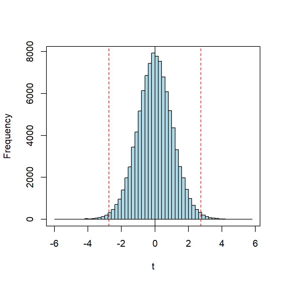

Figure 3.10: Monte Carlo t-distribution of sample size N=10 obtained by 100000 resampling steps from \(\sim N(0,1)\); the test value \(\pm 2.74\) in the present example is marked red in the plot.

prop.table(table(abs(t)>2.740403))

## 
##   FALSE    TRUE 
## 0.98688 0.01312

What does \(\alpha\) mean/tell?
It is the likelihood that a value larger than +2.74 or smaller than -2.74 will be observed under the Null-hypothesis H0, that is when there are truly no effects and both mean values, \(\bar x_{1,2}\), come from the same distribution.
\(\alpha\) is also called the False-Positive-Rate or Type-I Error Rate, the chance of taking an effect for real when it is not. In the present case \(\alpha\) is with \(\alpha = 0.01312\) very small, \(\approx 1\%\), and we tend to reject the Null-Hypothesis H0 in favour of the Alternative-Hypothesis H1 which states that there is a “true” underlying effect, and the underlying parameters \(\mu_{old},\mu_{new}\) are truly different. However, it must be kept in mind that \(\alpha = 0.01\) indicates a 1% chance that both processes are not different and potentially false-positive, so, ultimately, the test cannot and does not lead to certainty, but rather quantifies the certainty by reporting the False-Positive-Rate \(\alpha\). There are many tests in statistics such as, e.g., t-, F- and z-test, and they all come with the same logic:

1. One calculates from the data a statistics (a t-, F- or z-value, a real number).
2. One knows the distribution of the statistics under H0 and compares the statistics in hand with the distribution.
3. Depending on a preset decision level \(\alpha\) one either rejects or accepts the Null-Hypothesis H0 thereby accepting or rejecting the Alternative Hypothesis H1.

Usually there is no need to derive the test distribution by Monte Carlo simulation as virtually all important distributions are known in closed form and can be obtained analytically (however, Monte Carlo simulation has its place and is often the only method for deriving test distributions for non-normal data).
Figure 3.11 shows probability density plots of the t-distribution for different sample sizes. As a rule of thumb the t-distribution equals N(0,1) for N>30.

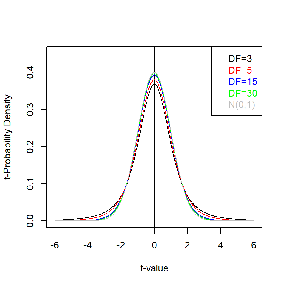
Figure 3.11: Probability density of the t-distribution, pdf(t|DF), for different degrees of freedom (DF)

Of course, there are ready-made functions for performing t-tests in all statistical software packages, in R, e.g., the base function t.test():

set.seed(1234)
old    <- rnorm(10,135,5)
new    <-  rnorm(10,140,5)
t.test(old,new, var.equal=T )

## 
##  Two Sample t-test
## 
## data:  old and new
## t = -2.7404, df = 18, p-value = 0.01344
## alternative hypothesis: true difference in means is not equal to 0
## 95 percent confidence interval:
##  -11.173926  -1.475941
## sample estimates:
## mean of x mean of y 
##  133.0842  139.4091

The t-tests reports an \(\alpha\)-value¹⁴ of 0.01344 in good agreement with the result obtained from Monte Carlo simulation. In addition the parameter df in the output reports the degrees of freedom, df=18, of the test. The t-test is based on two “internal” parameters, \(\bar X_{1}\) and \(\bar X_{2}\) and these two parameters must be deducted from the total sample size N=20, hence df=18¹⁵.
By convention a test result is called significant in statistics when \(0.01 \leq \alpha \leq 0.05\) and highly significant when \(\alpha < 0.01\).
When a test result is jugded significant given \(\alpha\), H0 is rejected in favour of H1 while silently accepting that in \(100*\alpha \%\) of the cases H0 will be true.
Similar to the error rate under H0, another error rate refering to H1 can be defined: The False-Negative-Rate \(\beta\) or the Type II Error Rate. Both error rates, \(\alpha\) and \(\beta\), are related with each other as figure 3.12 shows for the two sample t-test.

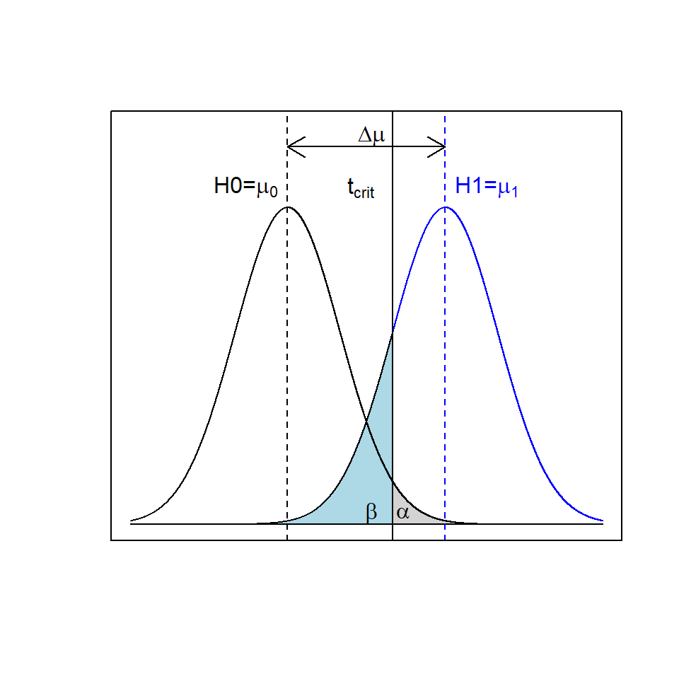
Figure 3.12: t-test and the relationship between \(\alpha\) (grey shaded area) and \(\beta\) (blue shaded area)

The False-Negative-Rate \(\beta\) is the likelihood of rejecting the Alternative-Hypothsis H1 when it is true. For instance, by increasing t_crit¹⁶ in 3.12 the likelihood \(\alpha\) for rejecting H0 in favour of H1 becomes very small at the expense of increasing \(\beta\). Small \(\alpha\)s (\(\Leftrightarrow\) large t_crit) will render decisions very conservative (rejecting most test results as nonresponders) to the detriment of accepting potential responders thereby inflating the likelihood \(\beta\). From an innovative point of view, \(\beta\) is much more important than \(\alpha\), because researchers usually want to identify responders rather than nonresponders. This naturally leads to the question whether it is possible to control both error rates simultaneously. It is, indeed, possible to control both error rates by appropriately choosing the sample size N_control and N_treat, as this will render both distributions, H0 and H1, wider or slender.
However, controlling \(\alpha\) and \(\beta\) requires knowledge about the effect size \(\Delta \mu\) and an estimate of \(\sigma\), see figure 3.12, a situation rarely given when analyzing historical data. Therefore, virtually all tests on happenstance data rely on \(\alpha\) with \(\beta\) unknown.
This situation changes when it comes to designed experiments, and that can be understood by recasting the t-test example from above: A researcher wants to set up an experiment with the current standard being \(135\pm5\). She considers an improvement of \(\Delta d=+5\) units economically worthwhile and wants to know the number of specimen for each group to ascertain an effect \(\Delta d\) given \(\alpha\) and \(\beta\). The following R-code answers this question (note that the effect size d is specified in standardized unit, that is \(d=\frac{\mu_{2}-\mu_{1}}{s}=\frac{140-135}{5}=1\); also note the definition power=1-\(\beta\)).

pwr::pwr.t.test(n = NULL, d = 1,sig.level = 0.05,
power = 0.9,alternative = c("greater"))

## 
##      Two-sample t test power calculation 
## 
##               n = 17.84712
##               d = 1
##       sig.level = 0.05
##           power = 0.9
##     alternative = greater
## 
## NOTE: n is number in *each* group

It takes 18 specimen in each group to ascertain an effect of \(\Delta=5\) with a pooled standard error of s=5 given \(\alpha=0.05\) and \(\beta=0.1\). If the test results after having performed the experiments turn out not significant (\(\alpha > 0.05\)) then the effect \(\Delta\) is very likely smaller than 5, hence the new process can be discarded as ineffective given \(\alpha=0.05\), \(\beta=0.1\). Of course, higher certainties, that is smaller \(\alpha\) and \(\beta\), will require larger sample sizes.
Depending on the experimental situation, researchers can tune \(\alpha\) and \(\beta\) according to their needs: If, for instance, the False-Positive-Rate hurts, which is typically the case in a later project phase with the product being closer to market, then \(\alpha\) should be made small. Conversely, when in an early project (screening) phase the False-Negative-Rate hurts. \(\alpha\) should be large and \(\beta\) comparatively small so as not to miss potential lead candidates.
Experimental designs simultaneously controlling \(\alpha\) and \(\beta\) are called powered designs and are the gold standard in the biomedical sciences.

3.4.2 Linear models and their use

In section 2.1 the elements of empirical model building were discussed starting with the base equation (3.5)

\[\begin{equation} \Delta y = f(\Delta X) + \epsilon = f(\Delta x_{1}, \Delta x_{2}... \Delta x_{I}) + \epsilon; \ \epsilon \sim N(0,\sigma^2) \tag{3.5} \end{equation}\]

Equation (3.5) creates the functional link between observed response \(\Delta y\) and the set of influential factors \(\Delta x_{1}, \Delta x_{2}... \Delta x_{I}\) augmented with uncertainty \(\epsilon\), with the latter, for good mathematical reasons (see chapter 2.1), assumed to come from a normal distribution with unknown variance \(\sigma^2\), that is \(\epsilon \sim N(0,\sigma^2)\). Unfortuantely, the function f() is unknown, however, can be locally approximated by low order polynomials of increasing complexity based on Taylor series expansion¹⁷.
Following this rationale, there are three levels of approximation of increasing complexity, namely the following three surrogate models

\[\begin{equation} f(\Delta x_{1}, \Delta x_{2}... \Delta x_{I}) \approx a_{0} + \sum_{i}a_{i}\cdot x_{i} \tag{3.6} \end{equation}\] \[\begin{equation} f(\Delta x_{1}, \Delta x_{2}... \Delta x_{I}) \approx a_{0} + \sum_{i}a_{i}\cdot x_{i} + \sum_{j>i}a_{ij}\cdot x_{i}\cdot x_{j} \tag{3.7} \end{equation}\] \[\begin{equation} f(\Delta x_{1}, \Delta x_{2}... \Delta x_{I}) \approx a_{0} + \sum_{i}a_{i}\cdot x_{i} + \sum_{i}a_{ii}\cdot x_{i}^2 + \sum_{j>i}a_{ij}\cdot x_{i}\cdot x_{j} \tag{3.8} \end{equation}\]

Surrogate model (3.6) is a linear model in x_i, whereas equation (3.7) denotes a bilinear model and (3.8) is a full second order model (often abbreviated RSM for Response Surface Model).
In the terminology of statistics, these surrogates are linear parametric models, because they are linear in the regression parameters a_i,a_ij although non-linear in the variables \(\Delta x_{1}, \Delta x_{2}... \Delta x_{I}\) (any model that can be written \(y = \sum_{j} a_{j}\cdot g_{j}(x_{1}\cdots x_{I})\) is linear in the regression parameters \(a_{j}\)). Contrary to linear models, the model \(\Delta y = a_{0} \cdot e^{a_{1}\cdot \Delta x}\) is non-linear in a₁ but can easily be linearized \(ln(\Delta y)=ln(a_{0}) + a_{1}\cdot \Delta x\). A non-linear parametric model which cannot be linearized is, e.g., the hyperbolic model \(\Delta y= \frac{1}{a_{0} + a_{1}\cdot \Delta x}\). It is important to keep linear and non-linear models apart as parameter estimation for non-linear models is more complex and not the subject of the present document. The topology of the three surrogate models in two dimensions is depicted in the figures 3.13, 3.14 and 3.15.

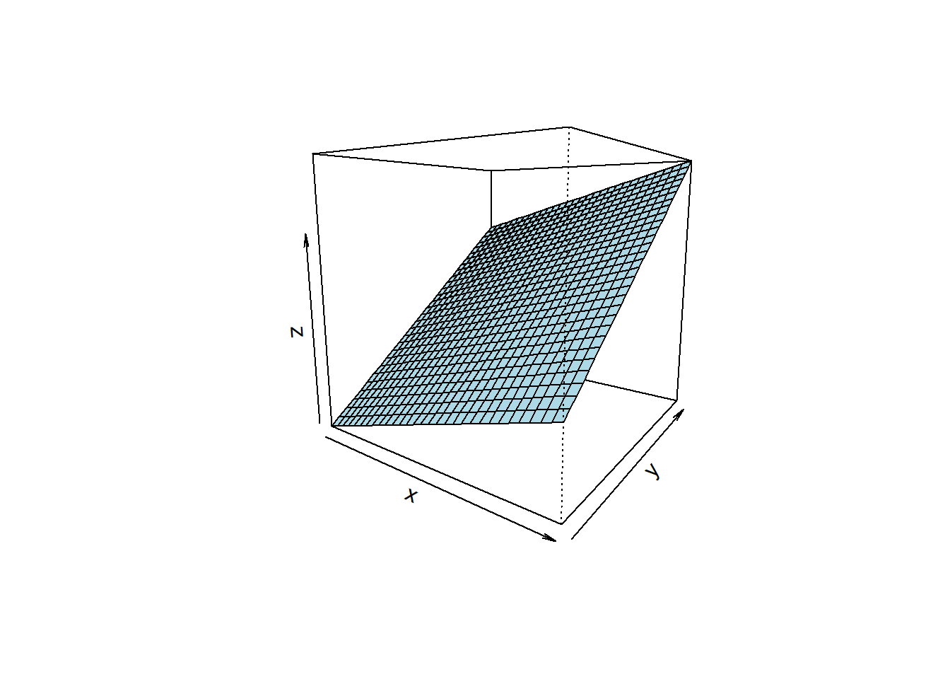
Figure 3.13: Linear parametric model \(z=a_{0} + a_{1} \cdot x + a_{2} \cdot y\).

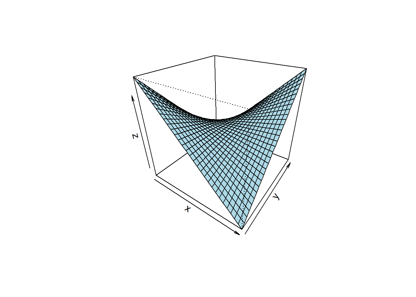
Figure 3.14: Bilinear parametric model \(z=a_{0} + a_{1} \cdot x + a_{2} \cdot y + a_{3} \cdot x \cdot y\).

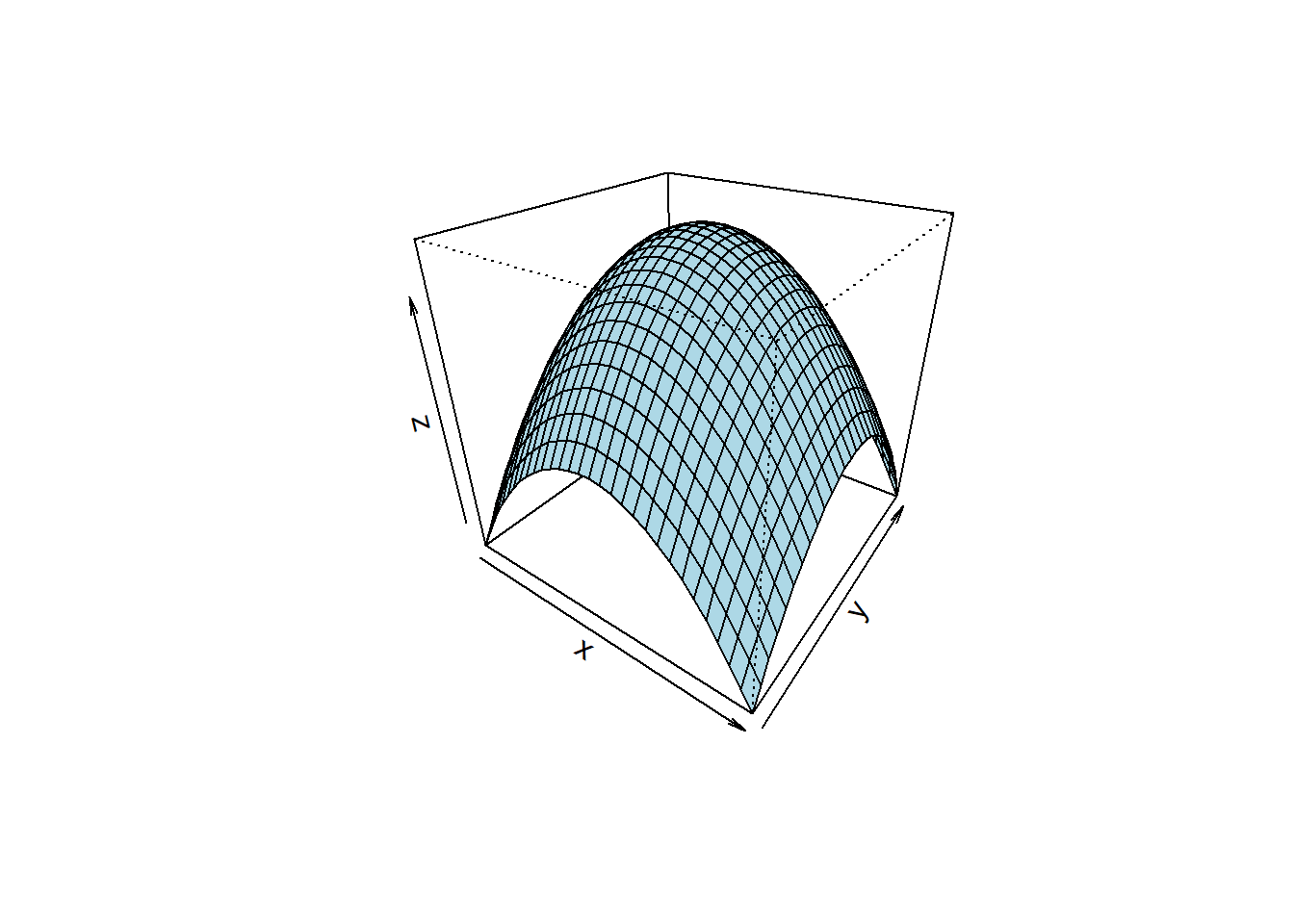
Figure 3.15: RSM model \(z=a_{0} + a_{1} \cdot x + a_{2} \cdot y + a_{3} \cdot x \cdot y + a_{4} \cdot x^2 + a_{5} \cdot y^2\).

Linear parametric models, equation (3.6), figure 3.13, describe planes and hyperplanes in \(\mathbb {R}\) with the effects given by the slope parameter \(a_{i}\). Linear models are often to simplistic by ignoring factor interactions, which, e.g., play an important role in the chemical sciences. Factor interactions can be accounted for by augmenting the linear model with bilinear model terms. As figure 3.14 shows, the effect of the factor x becomes dependent on y and vice versa. Given the bilinear equation \(y=a_{0} + a_{1}\cdot x_{1} + a_{2}\cdot x_{2} + a_{3}\cdot x_{1} \cdot x_{2}\), there are two potential readings, namely

1. \(y=a_{0} + (a_{1} + a_{3}\cdot x_{2})\cdot x_{1} + a_{2}\cdot x_{2}\)
2. \(y=a_{0} + a_{1}\cdot x_{1} + (a_{2} + a_{3}\cdot x_{1}) \cdot x_{2}\)

In the first reading the slope parameter of x₁ becomes a linear function of x₂, while in the second reading the slope of x₂ is being moderated by x₁ via parameter a₃. In high-dimensional space, \(\mathbb{R}\), bilinear models describe twisted planes or twisted hyperplanes.
Finally, response surface models can be used to describe local maxima, minima (see figure 3.15) or sattle points with the latter topology depicted in figure 3.16. Sattle points can make model interpretation and optimization more difficult as they show no clear direction of ascend or descend.

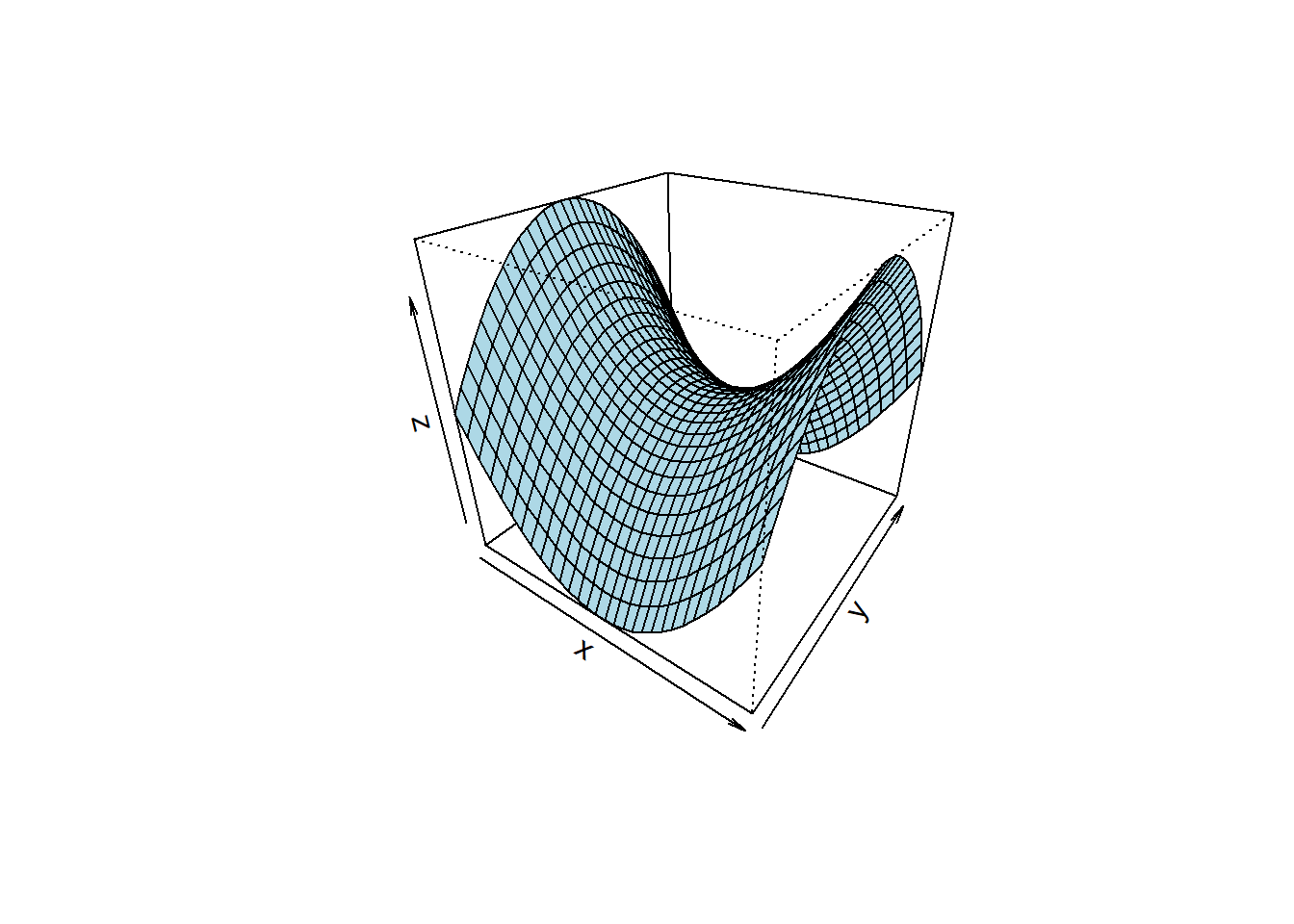
Figure 3.16: RSM model \(z=a_{0} + a_{1} \cdot x + a_{2} \cdot y + a_{3} \cdot x \cdot y + a_{4} \cdot (x^2 - y^2)\) revealing a sattle point.

It should be noted that it is usually impossible to infer the topology of the response surface alone from the analytical expression of the parametric model. As will be discussed later, there are mathematical techniques for converting RS-models into more “readable” models (canonical analysis). Alternatively, the response surface can be plotted as conditional RSM plots. However, the capability of the human mind for grasping high-dimensional visual information is limited, and mathematical techniques such as the aforementioned canonical analysis or optimization can simplify the analysis of high-dimensional models.

3.4.3 Least Squares in two dimensions

The key ideas of linear model buiding can be beneficially introduced with some low-dimensional (here: two-dimensional) examples based on simulated data. This has the advantage that the “true model” is known and that both, data and model, can be depicted in one plot.
As a first example, figure 3.17 shows a realization of 30 samples of the function \(y = 3 + 5\cdot x + \epsilon ; \space \epsilon \sim N(\mu = 0,\sigma=1)\)

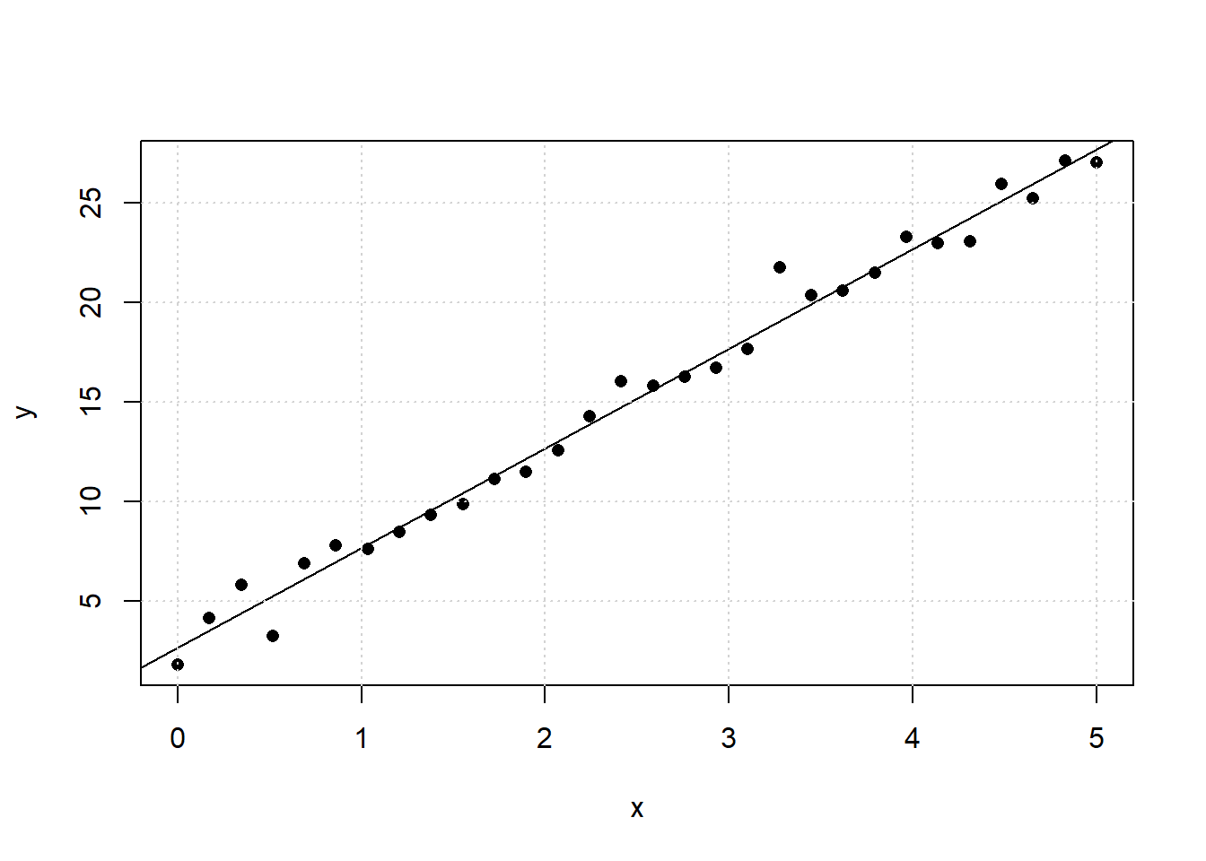
Figure 3.17: Simple scatter plot generated from the underlying function y = 3 + 5*x + N(0,1)

The linear regression line in figure 3.17 is the model estimate \(\hat y\) from a finite realization of the true, however unknown model \(y = 3 + 5\cdot x\). Model estimates from this realization can be obtained by drawing a straight line through the data with a ruler, so that the line fits the data “somehow well”. Of course, this process of “eye-ball regression” is not unique, subject to personal bias and is of only historical relevance. An objective and optimal method for estimating the unknown parameters a₀ and a₁ is the least squares technique invented by the German mathematician C.F. Gauss (1777-1855).
Least squares works by defining the Least Square objective function SS(a₀,a₁), the sum of squares, equation (3.9)

\[\begin{equation} SS(a_{0},a_{1}) = \sum_{i=1}^{N} (y_{i} - \hat y_{i} )^2 = \sum_{i=1}^{N} (y_{i} - [a_{0} + a_{1}\cdot x_{i}] )^2 \tag{3.9} \end{equation}\]

and minimizing SS(a₀,a₁) over a₀,a₁, that is \[\min_{a_{0},a_{1}} SS(a_{0},a_{1})\] The shape of SS(a₀,a₁) as a function of a₀,a₁ for the bivariate example above is shown in figure 3.18.

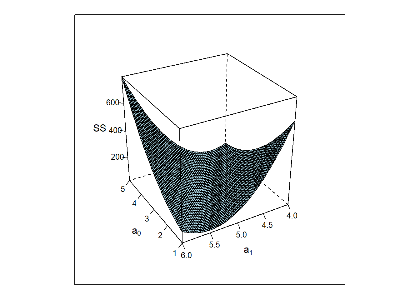
Figure 3.18: \(SS(a_{0},a_{1})\) as a function of \(a_{0}, a_{1}\) of sample size N=30 from \(y=3+5x + \epsilon; \epsilon \sim N(0,1)\).

Figure 3.18 reveals a convex shaped response surface with a flat minimum at \(a^*_{0} \approx 2.7\) and \(a^*_{1} \approx 5\). These results can be obtained analytically by equating the partial derivates of SS(a₀,a₁) with zero and solving for a₀,a₁, that is \[\frac {\partial SS(a_{0},a_{1}|y,x)} {\partial {a_{0}}} =0 \] \[ \frac {\partial SS(a_{0},a_{1}|y,x)} {\partial {a_{1}}} =0\] Solving the above normal equations gives the Least Squares solution for the bivariate case, namely \[a^*_{1} = \frac {\sum_{i=1}^{N}(y_{i} - \bar y) \cdot (x_{i} - \bar x)} {\sum_{i=1}^{N}(x_{i} - \bar x)^2} = \frac {\frac {1} {N-1} \sum_{i=1}^{N}(y_{i} - \bar y) \cdot (x_{i} - \bar x)} {\frac {1} {N-1} \sum_{i=1}^{N}(x_{i} - \bar x)^2} = \frac {Cov(y,x)} {Var(x)} \] \[ a^*_{0} = \bar y - a^*_{1} \cdot \bar x\] The optimal slope parameter is the ratio of the covariance of x and y divided by the variance of x. The sample covariance, equation (3.10), is a bivariate criterion for measuring the degree of linear association between two random variables.

\[\begin{equation} Cov(x,y) = {\frac {1} {N-1} \sum_{i=1}^{N}(y_{i} - \bar y) \cdot (x_{i} - \bar x)} \tag{3.10} \end{equation}\]

Being scale sensitive, the covariance is as such not very informative, but becomes more meaningful by scaling x and y appropriately, which leads to the well-known ordinary (or Pearson) correlation coefficient, equation (3.11) (the transformation \(x^*_{i} = \frac {x_{i} - \bar x} {s_x}\) has wide use in statistics and is commonly known as standardization and can be done in R with the base function scale()).

\[\begin{equation} Cor(x,y) = {\frac {1} {N-1} \sum_{i=1}^{N}( \frac {y_{i} - \bar y} {s_{y}}) \cdot ( \frac {x_{i} - \bar x} {s_{x}})} = \frac {1} {N-1} \sum_{i=1}^{N} y^*_{i}\cdot x^*_{i} = \frac {Cov(x,y)} {s_{x}\cdot s_{y}} \tag{3.11} \end{equation}\]

The Pearson correlation coefficient r_x,y is a scale free value in the range \(-1 \leq r_{x,y} \leq +1\) and tells how well the data fits the linear equation \(y = \hat y + \epsilon = a_{0} + a_{1}\cdot x + \epsilon\). Values of \(r_{x,y} = \pm 1\) indicate that the data fits the model \(\hat y\) with either positive or negative slope and \(\epsilon =0\). Values close to zero, \(|r_{x,y}| \approx 0\), indicate the absence of a linear relationship and suggest the random model \(y=\epsilon \ \forall \ x\).

Least Squares problems can be solved conveniently with statistical software, making Ordinary Least Squares (OLS) to the most widely used statistical method in science. In R the lm() function provides all functionalities for solving OLS problems, e.g. with the R example code

###### plot SS 
set.seed(1234)
x <- seq(0,5,length=30)
y <- 3 + 5*x + rnorm(length(x),0,1)
x.df <- data.frame(y,x) # make a data.frame
res <- lm(y~x,data=x.df) # do linear modeling
summary(res) # show results 

## 
## Call:
## lm(formula = y ~ x, data = x.df)
## 
## Residuals:
##     Min      1Q  Median      3Q     Max 
## -2.0306 -0.5751 -0.2109  0.5522  2.7050 
## 
## Coefficients:
##             Estimate Std. Error t value Pr(>|t|)    
## (Intercept)   2.6800     0.3273   8.188 6.51e-09 ***
## x             5.0094     0.1124  44.562  < 2e-16 ***
## ---
## Signif. codes:  0 '***' 0.001 '**' 0.01 '*' 0.05 '.' 0.1 ' ' 1
## 
## Residual standard error: 0.9189 on 28 degrees of freedom
## Multiple R-squared:  0.9861, Adjusted R-squared:  0.9856 
## F-statistic:  1986 on 1 and 28 DF,  p-value: < 2.2e-16

a1 <- cov(x,y)/var(x)              # analytical OLS solution 
a0 <- mean(y) - a1*mean(x)
c(a0=a0,a1=a1)                     # show OLS estimators a0,a1

##       a0       a1 
## 2.680009 5.009426

cor(x.df)                          # shows the Pearson  r.xy

##           y         x
## y 1.0000000 0.9930235
## x 0.9930235 1.0000000

sqrt(sum((y - predict(res))^2)/28) # residual standard error

## [1] 0.9188509

cor(x.df$y,predict(res))^2         # R2-value #1: cor(y,y.hat)^2; 

## [1] 0.9860958

ss <- anova(res)
names(ss)                          # what's in ss?

## [1] "Df"      "Sum Sq"  "Mean Sq" "F value" "Pr(>F)"

r2 <- ss[,2][1]/sum(ss[,2]) 
r2                              # R2-value #2: SS.model/ss.total

## [1] 0.9860958

F.test <- ss[,3][1]/ss[,3][2]   # Calculate F-value 
F.test

## [1] 1985.773

1-pf(F.test,ss[1,1],ss[1,2] )      # Prob(F>F.test)|H0

## [1] 0

The function lm() provides a lot of information and there are many ready-made auxiliary functions associated with objects of class “lm” such as plot.lm(), summary.lm(), predict.lm(),…, type “?lm” in the R console for more information.

3.4.3.1 OLS results and its interpretation

The output from summary(lm()) reports first OLS parameter estimates along with their corresponding standard errors (uncertainty), here \(a_{0} = 2.6800 \pm 0.3273\) and \(a_{1} = 5.0094 \pm 0.1124\). When the numerical range \(\hat a_{i} \pm 2\cdot \Delta a_{i}\) includes zero then, as a rule of thumb, the OLS parameters are noninformative and should be excluded from the model¹⁸. Underlying the two-sigma rule is a t-test with the statistics \(t=\frac {\hat a_{i}} {\Delta a_{i}}\). The t-values in the example, t₀=8.2 and t₁=44.6, exceed by far the critical 5% quantile of the t-distribution with 28 degrees of freedom¹⁹, here \(Prob(T>(t_{critical} = 0.51)|DF=28)=0.025\), and the Null-Hypothesis, \(a_{0}=0; a_{1}=0\) can safely be rejected in favour of H1, that is \(a_{0} \ne 0; a_{1} \ne 0\). The t-test statistics reported in the OLS output is a two-sided test and reports the probability \(Prob(|T|>t_{2})=\alpha\), the probability of finding a t-value larger or smaller than \(\pm t_{2}\) by chance under H0.
When the expected effect can be assumed positive (negative) a one-sided test, \(Prob(T>t_{1})=\alpha\), \((Prob(T< -t_{1})=\alpha)\), is more powerful, as t₁ < t₂ always holds given \(DF\) and \(\alpha\). Figure 3.19 schematically depicts how the one-sided relates to the two-sided test.
In the example, for instance, the likelihood that the test statistics \(t_{0}=\pm 8.2\) is exceeded or fallen short of under H0 is next to zero, more precisely Prob(|T|>8.2)=6.5*10^-9.

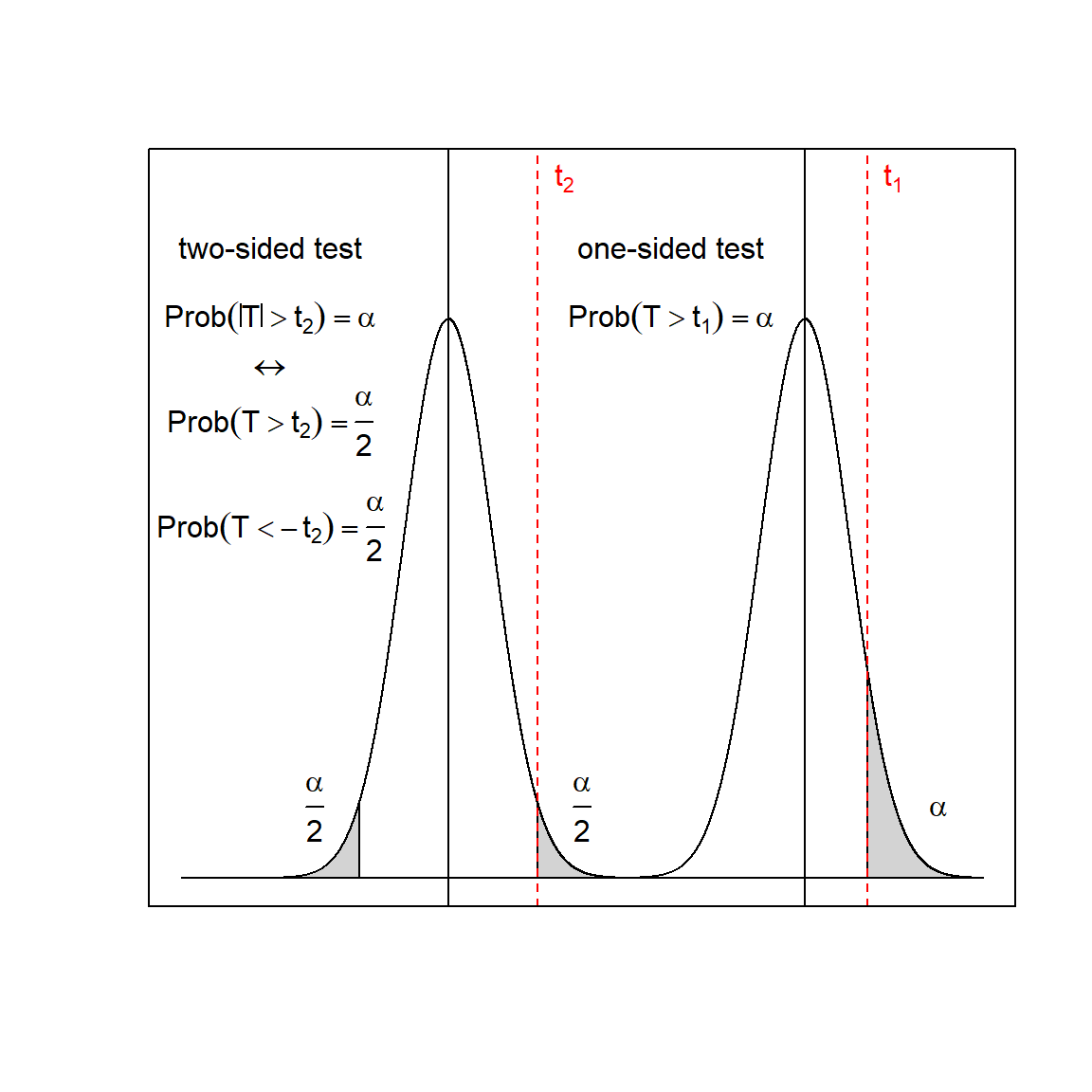
Figure 3.19: Two-sided and one-sided t-test given sample size N and test level \(\alpha\). Note that the decision threshold \(t_{2}\) for the two-sided test is larger than \(t_{1}\) rendering the two-sided test less powerful than the one-sided test

Next, the summary() function reports the residual standard deviation which is given by the expression, equation (3.12)

\[\begin{equation} s_{residual} = \sqrt{\frac {1}{N-p} \sum_{i=1}^{N}(y_{i} - \hat y_{i})^2} \tag{3.12} \end{equation}\]

with N denoting the number of observations and p the number of model parameters. The contrast (N-p) denotes the degrees of freedom (DF) of the linear model, for the bivariate example DF=(30-2)=28. \(s_{residual}\) is an unbiased estimate of the unknown standard error \(\sigma\) from the error term \(\epsilon ~\sim N(0,\sigma=1)\).
Next in the output follows the well-known R² value, which is defined in two different but mathematically equivalent ways.
The first definition is already suggested by the statistic’s name according to which R² is defined as the squared correlation coefficient between \(\hat y\) and \(y\), that is \(R^2 = Cor(\hat y,y)^2\). The second definition needs a little bit more elaboration and relies on the principle of partitioning the sum of squares, a principle that holds for all linear OLS models. According to this principle, the total sum of squares of the response y can be partioned into a model and an error part, see equation (3.13) and figure 3.20 for a graphical description.

\[\begin{align} \sum_{i=1}^{N} (y_{i}-\bar y)^2 \space\space & = \space\space \sum_{i=1}^{N} (\hat y_{i}-\bar y)^2 & + & \space\space\space\space \sum_{i=1}^{N} (y_{i}-\hat y_{i})^2 \notag \\ SS_{total} \space\space & = \space\space SS_{model} & + & \space\space\space\space SS_{error} \notag \\ (N-1) \space\space & = \space\space (p-1) & + & \space\space\space\space (N-p) \tag{3.13} \end{align}\]

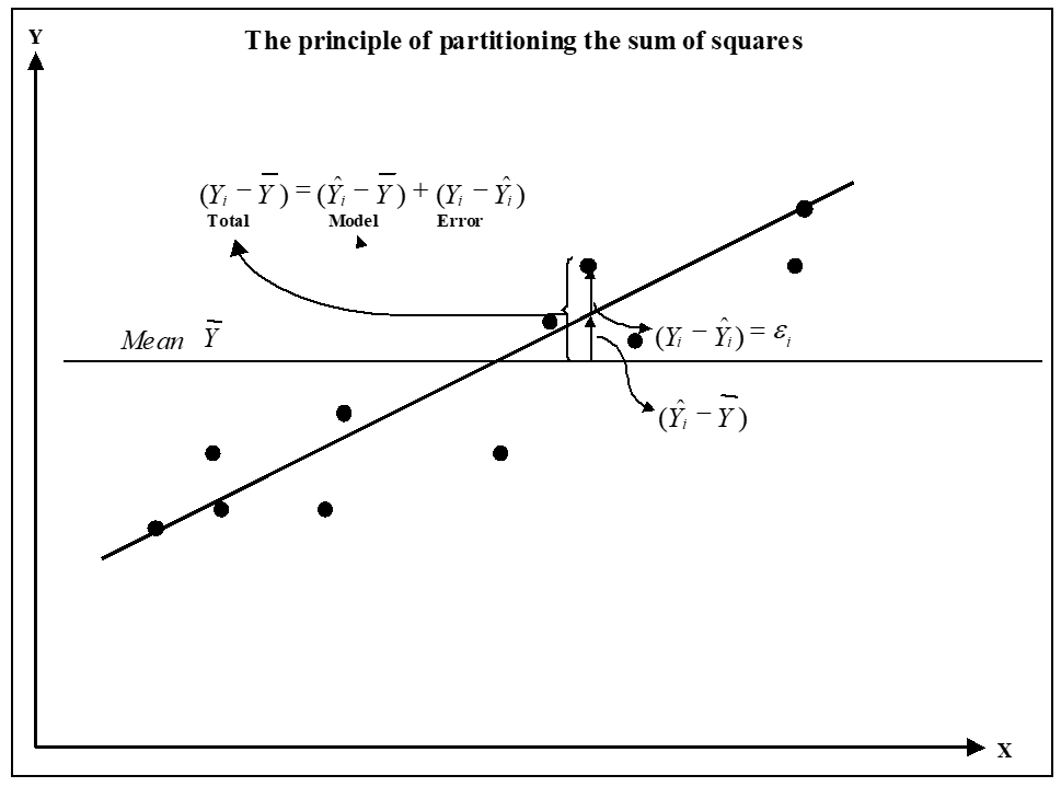
Figure 3.20: Partitioning the total sum of squares into model and error sum of squares

With both terms SS_total and SS_model from equation (3.13), the second definition of R² is simply \[R^2 = \frac {SS_{model}} {SS_{total}}=\frac {SS_{total} - SS_{error}} {SS_{total}}= 1 - \frac {SS_{error}}{SS_{total}}\] R² expresses the Goodness-of-Fit as the percentage of variance explained by the model and lies in the domain \(0 \leq R^2 \leq 1\). The elements of equation (3.13) give rise to another important statistics reported next in the lm-output, the F-statistics, named after the statistician R.A. Fisher.

\[\begin{equation} F = \frac {explained \ variance }{unexplained \ variance} = \frac {\frac {SS_{model} } {DF_{model} } } {{\frac {SS_{error} } {DF_{error} } }} = \frac {\frac {SS_{model} } {p-1} } {{\frac {SS_{error} } {N-p} }} \tag{3.14} \end{equation}\]

The F-statistics, equation (3.14), is a signal-to-noise ratio in the range \(0 \leq F \leq \infty\) and tests the global Null-hypothis against the global alternative H1,

\[\begin{align} H0 &: y = \epsilon \notag \\ H1 &: y = \hat y + \epsilon \tag{3.15} \end{align}\]

The F-test follows the test logic already discussed: The two-parametric distribution of F is known under the Null-Hypothesis H0, and the F-value obtained from the data, f_test, is compared against the F-distribution under H0, i.e. it is checked whether Prob(F>f_test|DF_model,DF_error) < 0.05 holds. If so, reject \(y=\epsilon\) in favour of \(y = f(X) + \epsilon\). Figure 3.21 shows the probability density of the F-distribution for different values of DF_model and DF_error.

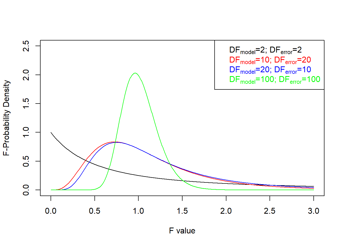
Figure 3.21: Probability density of the F-distribution for different parameters \(DF_{model}, DF_{error}\).

The F-value in the present example is reported to be F_test=1986 and the probability of observing such a large value is virually zero and H1 is accepted, so SS_model significantly contributes to the variance of y.
There is a test hierarchy: The F-test checks whether the model \(\hat y\) is different from 0 (tests, whether the model as a whole is significant), while the t-test checks whether the underlying regression parameters are significant. When the F-test turns out nonsignicant there is not much use checking the significance of the underlying regression parameters. However, there are cases where the F-test is significant with no regression parameter found significant. Such pathological cases can be informative in itself and will be discussed later.

3.4.3.2 Linear OLS for categorial data

In the above OLS example, response y and variable x were both of numerical data type and measured on a continuous, numerical scale. However, in the real world sciences there are a plethora of situations were some, if not all factors X belong to the categorial data type. For instance, a chemist might be interested in testing the performance of three different catalysts with the categorial levels Cat₁, Cat₂ and Cat₃ by setting up and analysing a categorial design.
It is in fact very easy to translate categorial variables into variables more amenable to numerical OLS analysis with the method called “dummy-coding”.
In order to understand this method, the t-test example from chapter 3.4.1 will be revisited and reformulated as a linear OLS model. The two samples from above are first converted into the data frame depicted in table 3.7 comprising 20 observations and two variables, namely the response “y” and the categorial treatment factor “treat” on the levels “old” and “new”.

Table 3.7: t-test data casted as a data frame of dimension 20x2

obsnr	treat	y
1	old	128.96
2	old	136.39
3	old	140.42
4	old	123.27
5	old	137.15
6	old	137.53
7	old	132.13
8	old	132.27
9	old	132.18
10	old	130.55
11	new	137.61
12	new	135.01
13	new	136.12
14	new	140.32
15	new	144.80
16	new	139.45
17	new	137.44
18	new	135.44
19	new	135.81
20	new	152.08

The idea of “dummy-coding” now consist in converting a factor with N categorial levels into N binary variables with numerical level 0/1. Table 3.8 shows the converted data frame together with the original data. Whenever the factor “treat” is on the level “old” then old=1; else old=0, and the same applies to the level “new”.

Table 3.8: Augmented t-test data with treat being dummy-coded as binary factors old, new

obsnr	treat	y	intercept	new	old
1	old	128.96	1	0	1
2	old	136.39	1	0	1
3	old	140.42	1	0	1
4	old	123.27	1	0	1
5	old	137.15	1	0	1
6	old	137.53	1	0	1
7	old	132.13	1	0	1
8	old	132.27	1	0	1
9	old	132.18	1	0	1
10	old	130.55	1	0	1
11	new	137.61	1	1	0
12	new	135.01	1	1	0
13	new	136.12	1	1	0
14	new	140.32	1	1	0
15	new	144.80	1	1	0
16	new	139.45	1	1	0
17	new	137.44	1	1	0
18	new	135.44	1	1	0
19	new	135.81	1	1	0
20	new	152.08	1	1	0

The data frame, table 3.8, suggest to set up the linear OLS model \(y=a_{0}\cdot intercept + a_{1}\cdot old + a_{2}\cdot new\) However, this linear model is overparametrized due to the equality constraint intercept= old + new=1. With the latter equality constraint the model can be rewritten \[ y=a_{0}\cdot intercept + a_{1}\cdot old + a_{2}\cdot new; \ intercept = old + new \Rightarrow \] \[ a_{0}\cdot intercept + a_{1}\cdot (intercept- new) + a_{2}\cdot new = \] \[ (a_{0} + a_{1})\cdot intercept + (a_{2} - a_{1})\cdot new = \\a^{'}_{0} \cdot intercept + \Delta a\cdot new \] From comparision follows, that by omitting the variable old from the regression equation \(y=a_{0}\cdot intercept + a_{1}\cdot old + a_{2}\cdot new\) the coefficient \(a_{2}\) becomes the contrast \(a_{2}-a_{1}\). Estimating and testing this contrast will directly answer the hypothesis at stake whether both treatments are the same or different.
The rule just derived holds for all categorial factors: Say, we have a 4-level factor with factor levels A₁, A₂, A₃, A₄: By dropping one level, A₂, all other levels turn into contrasts, here (A₁ - A₂), (A₃ - A₂) and (A₄ - A₂).
The factor levels to be dropped are typically the control (reference) levels of an experiment (in the t-test example the level “old”), and R by default assumes always the first level to be the reference (in the example the lexical order is “new”, “old”, hence the default reference is “new”). However, this default option can be overwritten by specifying the reference level explicitly with a reference option (see the R-example code).
The R-code for estimating and testing the contrast (new-old) with OLS then becomes

set.seed(1234)
rm(list=ls())
set.seed(1234)
old    <- rnorm(10,135,5)
new    <-  rnorm(10,140,5)

x <- data.frame(obsnr=1:20,treat=c(rep("old",10), 
                      rep("new",10) ), y=round(c(old,new),2))
levels(x$treat) # wrong order with "new" being the reference

## [1] "new" "old"

x$treat <- relevel(x$treat,ref="old") #.. so relevel
levels(x$treat)

## [1] "old" "new"

summary(lm(y~treat,data=x))

## 
## Call:
## lm(formula = y ~ treat, data = x)
## 
## Residuals:
##    Min     1Q Median     3Q    Max 
## -9.815 -3.365 -0.930  3.495 12.672 
## 
## Coefficients:
##             Estimate Std. Error t value Pr(>|t|)    
## (Intercept)  133.085      1.632  81.530   <2e-16 ***
## treatnew       6.323      2.308   2.739   0.0135 *  
## ---
## Signif. codes:  0 '***' 0.001 '**' 0.01 '*' 0.05 '.' 0.1 ' ' 1
## 
## Residual standard error: 5.162 on 18 degrees of freedom
## Multiple R-squared:  0.2942, Adjusted R-squared:  0.255 
## F-statistic: 7.502 on 1 and 18 DF,  p-value: 0.01348

The results are numerically the same as those obtained with the t-test, namely t=2.7404 and p-value=0.01344, and the OLS t-value is estimated to be \(t = 2.739\), which is significant at the 1.35% test level. The OLS-contrast is reported to be \(a_{new}-a_{old}=6.323\pm2.308\). Note, that the label of the OLS estimate treatnew denotes implicitly the contrast treatnew-treatold by convention.

3.4.3.3 OLS model diagnostic and violation of OLS assumptions

Model diagnostics, the process of comparing model predictions \(\hat y\) with the actually observed values \(y\), is an important step in the process of empirical model building. This seems trivial in the bivariate case y~f(x), where a simple scatter plot can depict both data \(y \sim x\) and model \(\hat y \sim x\) and thereby highlighting anomalies such as outliers or lack of fit. However, high-dimensional parametric models, \(\hat y = f(x_{1}, x_{2}...x_{I}|(a_{1},a_{2}...a_{K}))\) cannot be visualized together with the data underlying the models, and residual diagnostics become an important step for assessing Goodness-of-Fit and model quality.
From the parametric model equation \[y = f(x_{1}, x_{2}...x_{I}|(a_{1},a_{2}...a_{K})) + \epsilon; \ \epsilon \sim N(0,\sigma)\] follows directly the equation defining the residual \[\epsilon = y - f(x_{1}, x_{2}...x_{I}|(a_{1},a_{2}...a_{K}))\] The difference between observed response y and model expectation \(\hat y\), \[r_{i} = y_{i} - \hat y_{i}\] is the residual, which is assumed to come from a normal distribution. The purpose of residual analysis is to check whether this assumption is correct. Basically, there are three distributional assumptions of \(N(0,\sigma)\), also known as the Gauss-Markov (GM) conditions, which needs to be checked:

1. The expectation \(E()\) (the mean) of the error term should be zero, \(E(\epsilon)=0\), i.e. the residual should be free from outliers biasing the expectation of \(\epsilon\).
2. The variance of the error term should be constant, \(Var(\epsilon)=\sigma_{X}^2=const.\forall X\). The uncertainty should not be a function of the experimental space X, i.e. should be constant over experimental space. This property is called homoscedasticity in statistics.
3. \(E(\epsilon_{t}\cdot \epsilon_{t+i})=0; \forall i>0\), that is the error term \(\epsilon\) should be serially independent, i.e. uncorrelated in time, and from knowing \(\epsilon_{t_{0}}\) it should not be possible to forecast \(\epsilon_{t_{1}}\) with \(t_{1}>t_{0}\).

Checking whether the GM conditions hold is usually done graphically with three different plots:

1. Plot of the residual \(y - \hat y\) versus model expectation \(\hat y\).
2. Plot of the residual \(y - \hat y\) versus run order.
3. Plot of the autocorrelation function (ACF) \(r_{i}=E(\epsilon_{t} \cdot \epsilon_{t-i})\)

The first plot typically highlights Lack of Fit, outliers and inhomogeneous error variance, while the second and third plots aim at detecting seriell anomalies. Because the residuals are scale sensitive and on the same scale as the response y, they are usually standardized with an estimate of \(\sigma\) and the standardized residual follows \(r.studentized = \frac {y-\hat y} {\sigma}\). From normal probability theory it is known that 95% (99%) of the residuals can be expected to lie within the range of \(\pm 2\) (\(\pm 3\)) standard deviation under H0. Working with standardized residuals simplifies residual diagnostics as potential outliers can be scrutinized in a statistical meaningful contexts.
The autocorrelation function (ACF), \(\gamma_{\tau}\), of the residuals should be zero within standard error under the assumption of serial independence for all i>0. With R being the residual vector of length N the autocorrelation is defined \[\gamma_{\tau}=\sum_{i=1}^N\frac{(R_{i}-\mu)\cdot (R_{i+\tau}-\mu)}{\sigma_{R}^2}\] with \(\mu=E(R)\) and \(\sigma_{R}^2=Var(R)\).
The autocorrelation function is the correlation coefficient betweeen \(\tau\)-lagged residual terms, \(cor(R_{t},R_{t+\tau} )\) and can be expected to be zero under serial independence. Figure 3.22 shows a simulated example violating the first GM condition by two outliers. Outliers are a reality in empirical data and might reflect a lack of experimental control or alternatively model inadequacy, i.e. a non-linearity not approriately described by the empirical model. Depending on the objective of the project²⁰, outlier should be checked by repeating the outlying experiments.

set.seed(1234)
x <- seq(0,5,length=30)
XX <- as.matrix(cbind(1,x))
y <- 3 + 5*x + rnorm(length(x),0,5)
y[x > 3.8 & x < 4.2] <- y[x > 3.8 & x < 4.2] - 25
res <- lm(y~x)

layout(matrix(c(1,2,3,4), 2, 2, byrow = TRUE))
plot(x,y,type="n",pch=16, ylim=c(-20,40), main="y~x")
text(x,y,label=1:length(y))
abline(lm(y~x)$coef)
grid()
plot(predict(res), rstudent(res),xlab=expression( paste("predicted response ", hat(y)) ) ,ylim=c(-5,3)   ,
     ylab="studentized residuals",type="n",
     main=expression(paste("(",frac(paste("y - ", hat(y)),sigma), ") ~ ", hat(y)   )) )

text(predict(res), rstudent(res),label=1:length(y))
abline(h=c(-2,0,2),lty=c(2,1,2))
grid()
plot(1:length(y), rstudent(res),xlab="run order",ylab="studentized residuals",type="l",
     main=expression(paste("(",frac(paste("y - ", hat(y)),sigma), ") ~ run order"   )))
abline(h=c(-2,0,2),lty=c(2,1,2))
grid()
acf(rstudent(res), main="Autocorrelation function of residuals")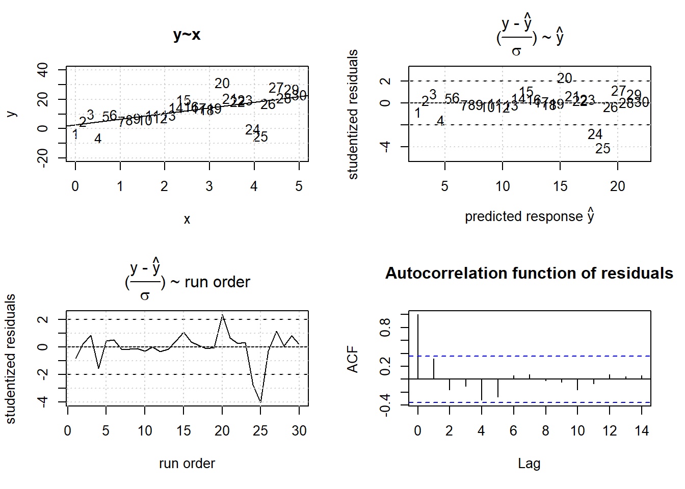

Figure 3.22: Effects of outlying observations on OLS estimation.

summary(res)

## 
## Call:
## lm(formula = y ~ x)
## 
## Residuals:
##      Min       1Q   Median       3Q      Max 
## -23.4949  -1.3215   0.6568   3.2538  16.0924 
## 
## Coefficients:
##             Estimate Std. Error t value Pr(>|t|)    
## (Intercept)   2.6366     2.6802   0.984 0.333666    
## x             3.8858     0.9205   4.221 0.000232 ***
## ---
## Signif. codes:  0 '***' 0.001 '**' 0.01 '*' 0.05 '.' 0.1 ' ' 1
## 
## Residual standard error: 7.524 on 28 degrees of freedom
## Multiple R-squared:  0.3889, Adjusted R-squared:  0.3671 
## F-statistic: 17.82 on 1 and 28 DF,  p-value: 0.0002315

The outlying observations #24, #25 stick out by four standard deviations (#20 being a borderline case), which is under normality, H0, very unlikely. The slope parameter of the “true” model \(y = 3 + 5*x + N(0,5)\) is estimated to be \(a_{1}=3.9\pm 0.9\), which is, despite the outliers, in good accordance with the true value. Hence, the slope bias incurred by the two outliers is in this example small. However, the true value \(\sigma=5\) of the error term \(\epsilon\) is with \(s_{residual}=7.5\) significantly overestimated.

The next simulation, figure 3.23, will demonstrate the effects of inhomogeneous variance on OLS model predictions (the R-code is skipped for brevity and only lm-results are being printed). The underlying model is \(y = 3 + 5 \cdot x + N(0,4\cdot x)\) and severely heteroscedastic with the variance proportional to x, \(\sigma=4 \cdot x\).

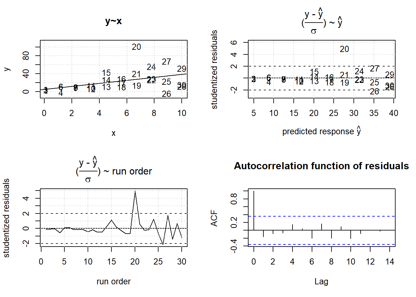
Figure 3.23: Effects of heterogenous variance on OLS

## 
## Call:
## lm(formula = y ~ x)
## 
## Residuals:
##     Min      1Q  Median      3Q     Max 
## -39.247  -9.574  -3.125   4.152  73.598 
## 
## Coefficients:
##             Estimate Std. Error t value Pr(>|t|)   
## (Intercept)    4.670      7.074   0.660   0.5146   
## x              3.429      1.188   2.888   0.0074 **
## ---
## Signif. codes:  0 '***' 0.001 '**' 0.01 '*' 0.05 '.' 0.1 ' ' 1
## 
## Residual standard error: 20.55 on 28 degrees of freedom
## Multiple R-squared:  0.2295, Adjusted R-squared:  0.202 
## F-statistic: 8.339 on 1 and 28 DF,  p-value: 0.007402

While the OLS parameter estimates agree very well with the true values \(a_{0}=3; \ a_{1}=5\) within standard error, the scatter plot y~x reveals the model prediction to be biased. The high precision observations in the lower x-range {0,4} are not properly met by the regression line with the regression line being above the data points. This results from the fact that the OLS objective function \(\sum_{i}(y_{i}-\hat y_{i})^2\) gives each observation equal weight. However, observations with small standard deviation should get higher weight, while high variance observation should receive a lower weight in the least square functional.

Unbiased OLS estimates can be obtained by using the standard deviation of each replication triple s_i for defining a weighted least squares function, \(\sum_{i} \frac {(y_{i} - \hat y_{i})^2} {s_{i}^2}\).

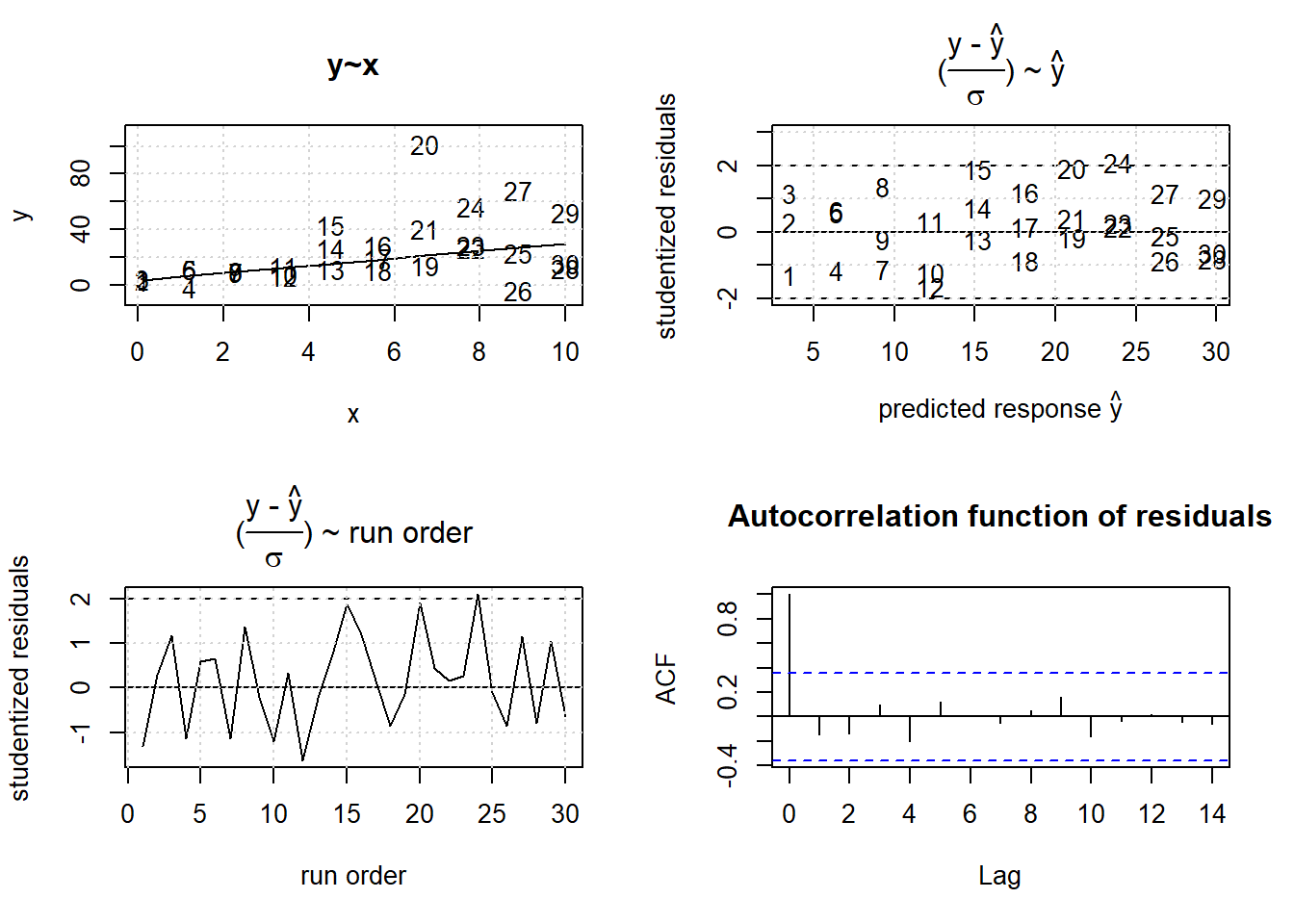
Figure 3.24: WLS results with weights inversely equal to the variance of the observation, \(w_{i}=\frac{1}{s_{i}^2}\)

## 
## Call:
## lm(formula = y ~ x, weights = wls)
## 
## Weighted Residuals:
##     Min      1Q  Median      3Q     Max 
## -1.5571 -0.7522  0.2036  0.8851  1.9438 
## 
## Coefficients:
##             Estimate Std. Error t value Pr(>|t|)    
## (Intercept)   3.2341     0.2727   11.86 1.96e-12 ***
## x             2.6506     0.1229   21.57  < 2e-16 ***
## ---
## Signif. codes:  0 '***' 0.001 '**' 0.01 '*' 0.05 '.' 0.1 ' ' 1
## 
## Residual standard error: 0.9832 on 28 degrees of freedom
## Multiple R-squared:  0.9432, Adjusted R-squared:  0.9412 
## F-statistic: 465.1 on 1 and 28 DF,  p-value: < 2.2e-16

The residuals in figure 3.24 agree very well with the pattern expected under normality, and the WLS model now describes the data within error unbiasedly.
Heterogeneity of variance is often observed in the real sciences. In chemistry, for instance, the accuracy of instruments are often specified as a percentage of the measured response thereby rendering the variance non-constant over measurement range. WLS is a versatile instrument for dealing with heterogeneous variance. Alternatively, a logarithmic transformation of the the response can sometimes stabilize the variance. The log-transformation will stretch small values and compress large values thereby giving small values higher and large values lower weight.

The third GM condition refers to the assumption of serial independence, that is \(E(\epsilon_{t}\cdot \epsilon_{t+i})=0; \forall i>0\). The most serious violation of this assumption is obtained by artficially replicating (copying) observations. By creating copies, say duplicates, the corresponding error terms \(\epsilon_{1} , \epsilon_{2}\) will be identical thus creating “fake” precision. Rather than two there is in reality only one degree of freedom causing the OLS test statistics to become very liberal (reporting significance by underestimating the standard error when in reality there is no significance). The residual plot, r ~(run order), in figure 3.25 reveals the residuals to be associated with its predecessor in time, here positively autocorrelated²¹. The data was created from the model \(y=3 + 5 \cdot x + \epsilon_{t};\ \epsilon_{t}=a_{1} \cdot \epsilon_{t-1} + \epsilon_{0};\ \epsilon_{0} \sim N(0,\sigma=5)\)
In the real world positive autocorrelation often results from oversampling a process by increasing the sampling rate beyond reasonable limits, in this way creating lots of data, essentially copies, with little information content.
The method of generalized least squares (GLS) can deal with autocorrelated data and yield unbiased estimates and test statistics. However, GLS is beyond the scope of this document and will not be considerred any further here. A simple trick for dealing with autocorrelations is to mean aggregate dependent observations. By the Central Limit Theorem, the resulting mean values will be closer to normality and serial independence. In DoE autocorrelation is seen rarely as the sample size is usually too small for rendering these effects detectable. Serial effects in DoE often indicate systematic effects in time such as loss of catalytic activity or deterioration of analytical instruments.

set.seed(1234)
x <- seq(0,5,length=30)
y <- 3 + 5*x + 5*arima.sim(list(ar=c(0.95)),30)
res <- lm(y~x)
layout(matrix(c(1,2,3,4), 2, 2, byrow = TRUE))
plot(x,y,type="n",pch=16, ylim=c(0,50), main="y~x")
text(x,y,label=1:length(y))
abline(lm(y~x)$coef)
grid()
plot(predict(res), rstudent(res),xlab=expression( paste("predicted response ", hat(y)) ) ,ylim=c(-3,3)   ,
     ylab="studentized residuals",type="n",
     main=expression(paste("(",frac(paste("y - ", hat(y)),sigma), ") ~ ", hat(y)   )) )
text(predict(res), rstudent(res),label=1:length(y))
abline(h=c(-2,0,2),lty=c(2,1,2))
grid()
plot(1:length(y), rstudent(res),xlab="run order",ylab="studentized residuals",type="l",ylim=c(-3,3)   ,
     main=expression(paste("(",frac(paste("y - ", hat(y)),sigma), ") ~ run order"   )))
abline(h=c(-2,0,2),lty=c(2,1,2))
grid()
acf(rstudent(res), main="Autocorrelation function of residuals")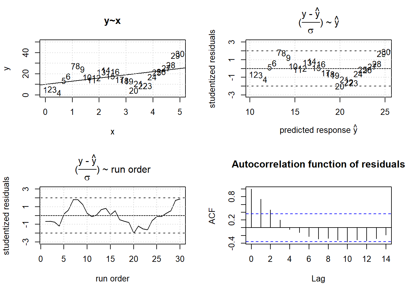

Figure 3.25: OLS results with positively autocorrelated error

summary(res)

## 
## Call:
## lm(formula = y ~ x)
## 
## Residuals:
##      Min       1Q   Median       3Q      Max 
## -15.3957  -5.2302  -0.2657   4.9561  14.1255 
## 
## Coefficients:
##             Estimate Std. Error t value Pr(>|t|)   
## (Intercept)   10.152      2.960   3.430  0.00189 **
## x              2.988      1.017   2.939  0.00653 **
## ---
## Signif. codes:  0 '***' 0.001 '**' 0.01 '*' 0.05 '.' 0.1 ' ' 1
## 
## Residual standard error: 8.31 on 28 degrees of freedom
## Multiple R-squared:  0.2357, Adjusted R-squared:  0.2084 
## F-statistic: 8.637 on 1 and 28 DF,  p-value: 0.006531

The examples considered so far all refer to anomalies in the error term \(\epsilon\) of \(f(x_{1},x_{2}...x_{I}|a_{1},a_{2}...a_{K}) + \epsilon\) which show up as non-normality in the residuals.
However, anomalies in the residuals can also arise from misspecifying the functional part f() in \(f(x_{1},x_{2}...x_{I}|a_{1},a_{2}...a_{K}) + \epsilon\).
The example data depicted in figure 3.26 is a realization of the model \(y=3+5 \cdot x + 3 \cdot x^2 + \epsilon; \ \epsilon \sim N(0,5)\) analyzed with the parametric OLS model \(y=a_{0} + a_{1} \cdot x\).

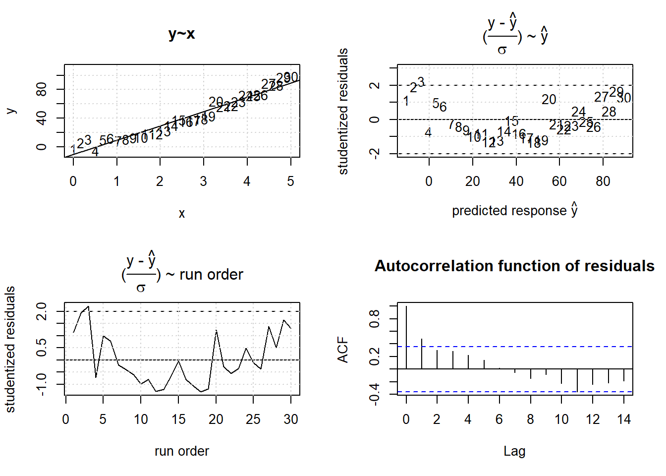
Figure 3.26: Linear, \(\hat y=a_{0} +a_{1} \cdot x + \epsilon\), OLS results from non-linear data, \(y=a_{0} +a_{1} \cdot x + a_{2} \cdot x^2 + \epsilon\).

## 
## Call:
## lm(formula = y ~ x)
## 
## Residuals:
##    Min     1Q Median     3Q    Max 
## -9.218 -5.559 -2.161  6.512 14.259 
## 
## Coefficients:
##             Estimate Std. Error t value Pr(>|t|)    
## (Intercept) -10.6689     2.5772   -4.14 0.000289 ***
## x            20.0471     0.8852   22.65  < 2e-16 ***
## ---
## Signif. codes:  0 '***' 0.001 '**' 0.01 '*' 0.05 '.' 0.1 ' ' 1
## 
## Residual standard error: 7.235 on 28 degrees of freedom
## Multiple R-squared:  0.9482, Adjusted R-squared:  0.9464 
## F-statistic: 512.9 on 1 and 28 DF,  p-value: < 2.2e-16

The residuals in figure 3.26 indicate that the model (the horizontal line in the residual plots at r_i=0) underestimates the data at the lower and upper tail, while overestimating the response y in the middle range. This is an indication of some non-linearity not accounted for by the linear model.
Remodeling the data with a quadratic RSM model \(y=a_{0} + a_{1} \cdot x + a_{2} \cdot x^2\) gives the result depicted in figure 3.27

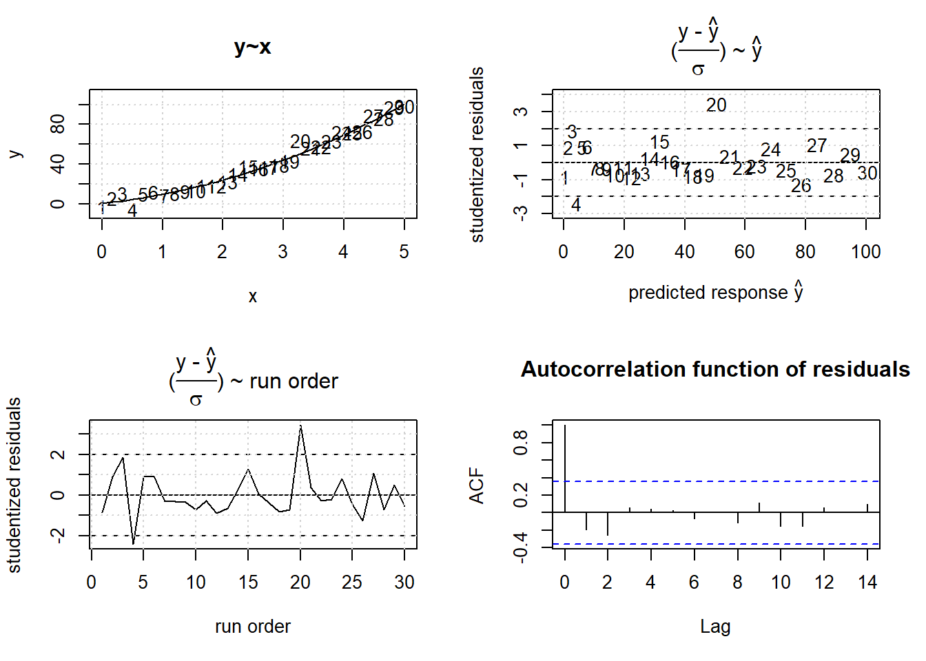
Figure 3.27: RSM results from non-linear data, \(y=a_{0} +a_{1} \cdot x + a_{2} \cdot x^2 + \epsilon\).

## 
## Call:
## lm(formula = y ~ x + I(x^2))
## 
## Residuals:
##    Min     1Q Median     3Q    Max 
## -9.691 -3.045 -1.324  3.308 13.084 
## 
## Coefficients:
##             Estimate Std. Error t value Pr(>|t|)    
## (Intercept)   0.3093     2.3829   0.130  0.89770    
## x             6.4028     2.2062   2.902  0.00729 ** 
## I(x^2)        2.7289     0.4264   6.400 7.42e-07 ***
## ---
## Signif. codes:  0 '***' 0.001 '**' 0.01 '*' 0.05 '.' 0.1 ' ' 1
## 
## Residual standard error: 4.644 on 27 degrees of freedom
## Multiple R-squared:  0.9794, Adjusted R-squared:  0.9779 
## F-statistic:   643 on 2 and 27 DF,  p-value: < 2.2e-16

Figure 3.27 does not reveal anomalies anymore and shows at the same time how the residuals should ideally look like, a homogeneous band with no systematic pattern in the range of \(\pm 3\cdot \sigma\). However, figure 3.27 should also be taken as a warning not to adhere too strictly to the \(\pm 3\sigma\) rule as the “outlier”, #20, is a chance result. So, unlikely things nevertheless happen.

3.4.3.4 OLS in many dimensions

In this section the low dimensional examples considered so far will be extended to higher dimensions. Given a data matrix of influential factors X with dimension Nxp (N times p) and a response vector of length N, the problem can be concisely expressed by equation (3.16)

\[\begin{equation} \mathbf {y} = \boldsymbol {X}{\boldsymbol {\beta }} + \boldsymbol {\epsilon} ; \epsilon \sim N(0,\sigma^2) \tag{3.16} \end{equation}\]

with the individual elements \(\boldsymbol X\), \(\boldsymbol y\) and \(\boldsymbol \beta\) given in (3.17)

\[\begin{equation} \displaystyle \boldsymbol {X} ={\begin{bmatrix}1;X_{11};X_{12};\cdots ;X_{1p}\\1;X_{21};X_{22};\cdots ;X_{2p}\\ \vdots \space\space\space\space\space\space \ddots \space\space\space\space\space\space \vdots \\1;X_{n1};X_{n2};\cdots ;X_{np}\end{bmatrix}},\qquad {\boldsymbol {\beta }}={\begin{bmatrix}\beta_{0}\\\beta _{1}\\\beta _{2}\\\vdots \\\beta _{p}\end{bmatrix}},\qquad \mathbf {y} ={\begin{bmatrix}y_{1}\\y_{2}\\\vdots \\y_{n}\end{bmatrix}} \tag{3.17} \end{equation}\]

Note that the data matrix has been augmented by a column of 1’s corresponding to the intercept parameter \(\beta_{0}\). Also note, that the data matrix \(\boldsymbol X\) also includes higher order model terms, here bilinear and/or quadratic terms, if these terms are specified in the formula expression of lm(). In R the model matrix is generated from the variables in a data frame and a symbolic formula (see “?formula”) by the function model.matrix(). When running lm() this function is implicitly called prior to parameter estimation.
The OLS solution \(\hat \beta\) can be derived by minimizing the quadratic norm, the function \(S(\beta)\) over \(\beta\) as shown in equation (3.18), something that can be done analytically by equating the partial derivatives with zero, \(\frac {\partial S} {\partial \beta_{i}}=0\) and solving for \(\beta\).

\[\begin{equation} {\displaystyle S({\boldsymbol {\beta }})={\bigl \|}\mathbf {y} -\mathbf {X} {\boldsymbol {\beta }}{\bigr \|}^{2} \\ {\hat {\boldsymbol {\beta }}}={\underset {\boldsymbol {\beta }}{\operatorname {arg\,min} }}\,S({\boldsymbol {\beta }}) } \tag{3.18} \end{equation}\]

Skipping the mathematical details here, the OLS solution is finally found by the equation (3.19)

\[\begin{equation} \boxed {\displaystyle {\hat {\boldsymbol {\beta }}}=(\mathbf {X} ^{\rm {T}}\mathbf {X} )^{-1}\mathbf {X} ^{\rm {T}}\mathbf {y}} \tag{3.19} \end{equation}\]

The computational burden of equation (3.19) is in essence the inversion of the covariance matrix \(\boldsymbol {X^T \cdot X}\), something that can be done in real time with modern computers. The OLS solution, equation (3.19), is a function of the random variable y and thereby becomes itself a random variable with expectation \(\hat \beta\) and variance, \(Var(\hat \beta)>0\).
It can be shown²² that \(Var(\hat \beta)\) is given by equation (3.20) which is the fundamental equation of experimental design.

\[\begin{equation} \boxed {\displaystyle \operatorname {Var} (\,{\hat {\beta }})=\sigma ^{2}(\boldsymbol {X^{T}X)^{-1}}} \tag{3.20} \end{equation}\]

In equation (3.20) the parameter \(\sigma^2\) affecting the error term is controlled by nature and basically not under the control of the experimenter (or only remotely under her control by keeping the ambient conditions as constant as possible, \(\rightarrow \Delta Z=0\)). However, the design matrix X affecting the variance of \(\hat \beta\) is under the control of the researcher.
Experimental design then becomes, very broadly stated, the process of designing X in such way that \(Var(\hat \beta)\), equation (3.20), attains a minimum within the experimental uncertainty, \(\sigma^2\), set by nature.

---

7. Smoothness of nature finds expression in the Latin phrase “Natura non facit saltus”: nature does not make jumps.↩

8. the difference between model #3 and #4 is especially important when it comes to finding conditions maximizing yield. #4 suggests a maximum in the present design space, while #3 points to a maximum somewhere outside this space.↩

9. of course time as such is not responsible for the observed correlation between storck and birth numbers. Living conditions of storcks and humans might have improved in the time range thereby creating the observed population trend.↩

10. r denotes the Pearson correlation coefficient. A value of +1 indicates that \(temp\) and \(time\) are perfectly colinear and their relationship can be expressed by the linear equation \(temp=b_{0} + b_{1}\cdot time\) with \(b_{1} > 0\).↩

11. Plant operators will certainly not be amused by suggesting to randomly increase and decrease the temperature over the course of the experimental programm. In addition, randomly varying the temperature can be a cause of catalytic activity loss.↩

12. There are many probability distributions in statistics but the normal distribution is by far the most important one as a result of the Central Limit Theorem: Sums of arbitrary distributed random variables will be asymptotically normal distributed, see the arguments from section 2.1.↩

13. For instance, it can be shown that the population mean of size N is normally distributed with \(N(\mu,\frac {s} {\sqrt{N}})\). As a consequence, a doubling of the precision, \(\frac {s}{2}\), requires quadrupling the experimental effort.↩

14. In statistics \(\alpha\)-values are often simply called p-values.↩

15. Informally speaking two data points were “consumed” for estimating \(\bar X_{1}\) and \(\bar X_{2}\) and are no longer available for the t-statistics.↩

16. The value t_crit is the decision boundary of the test. In the two sample t-test we obtain a test statistics t. If tt_crit we accept H1 and reject H0. By increasing t_crit \(\alpha\) becomes small at the expense of making \(\beta\) large (and vice-versa). In a minute we will an example where this property will be exploited for determining the optimal sample size of a t-test↩

17. Taylor series expansion requires the unknown function f() to be smooth and continuous↩

18. In a linear model \(\hat y=a_{0} + \sum_{i} a_{i} \cdot x_{i}\) non-significant parameters a_k will only inflate the variance of the model \(\hat y\), \(Var(\hat y)=\sum_{k} x_{k}^2 \cdot Var(a_{k})\) without significantly contributing any information to the model \(\hat y\). Therefore, non-significant factors x_k should be excluded from the model↩

19. The degrees of freedom, DF, are given by the equation DF=N-p, mit N being the number of observations and p being the number of estimated parameters. In the bivariate example a₀ and a₁ are being estimated from 30 observations, hence DF=28.↩

20. if, say, the objective is maximizing y and there is an outlier positively exceeding all other observations, this experiment should be and must be repeated, as the outlier could have resulted from some advantageous conditions X otherwise going unnoticed. This is of course not nescessary if the project goal is minimization.↩

21. Informally, positive autocorrelation is indicated by a “lack of scattering” and smoothness in the residual plots. Negative autocorrelation of the error term renders the residual plot very “spiky” and non-smooth. In chemistry, negative autocorrelation can result from carry-over-effects: A positive deviation (error) is followed by a negative deviation and so on. However, positive is far more common then negative autocorrelation.↩

22. see, for instance, (A. Sen, M. Srivastava 1990)↩