You have a brand new coin and you want to estimate \(p\), the probability that it lands on heads. You flip the coin \(n\) times and observe \(X\) heads.
Suggest an estimator of \(p\); it should be an expression involving \(X\) and \(n\). Describe in words what your estimator is. (Hint: what is the most obvious estimator you can think of?)
Suppose you observe \(x = 6\) heads in \(n=10\) flips. Use your estimator to compute an estimate of \(p\) based on this sample.
Consider the estimator (called the “plus four” estimator) \[
\frac{X + 2}{n + 4} = \left(\frac{4}{n+4}\right)\left(0.5\right) + \left(\frac{n}{n+4}\right)\left(\frac{X}{n}\right)
\] Explain in words what this estimator does. (The two expressions in the equation above are just different ways of expressing the estimator.)
Use the estimator from the previous part and compute an estimate of \(p\) based on a sample with 6 heads in 10 flips.
If you observe 6 heads in 10 flips, which of your two estimates is a better estimate of \(p\)? Explain.
Compute and interpret the probability of observing 6 heads in 10 flips if \(p = 0.6\).
Compute and intepret the probability of observing 6 heads in 10 flips if \(p = 0.571\).
Compare the values from the two previous parts. If you observed 6 heads in 10 flips, which of the values — 0.6 or 0.571 — would you choose as your estimate of \(p\)? Explain your reasoning.
Suppose you observe 6 heads in 10 flips. Carefully write the likelihood function.
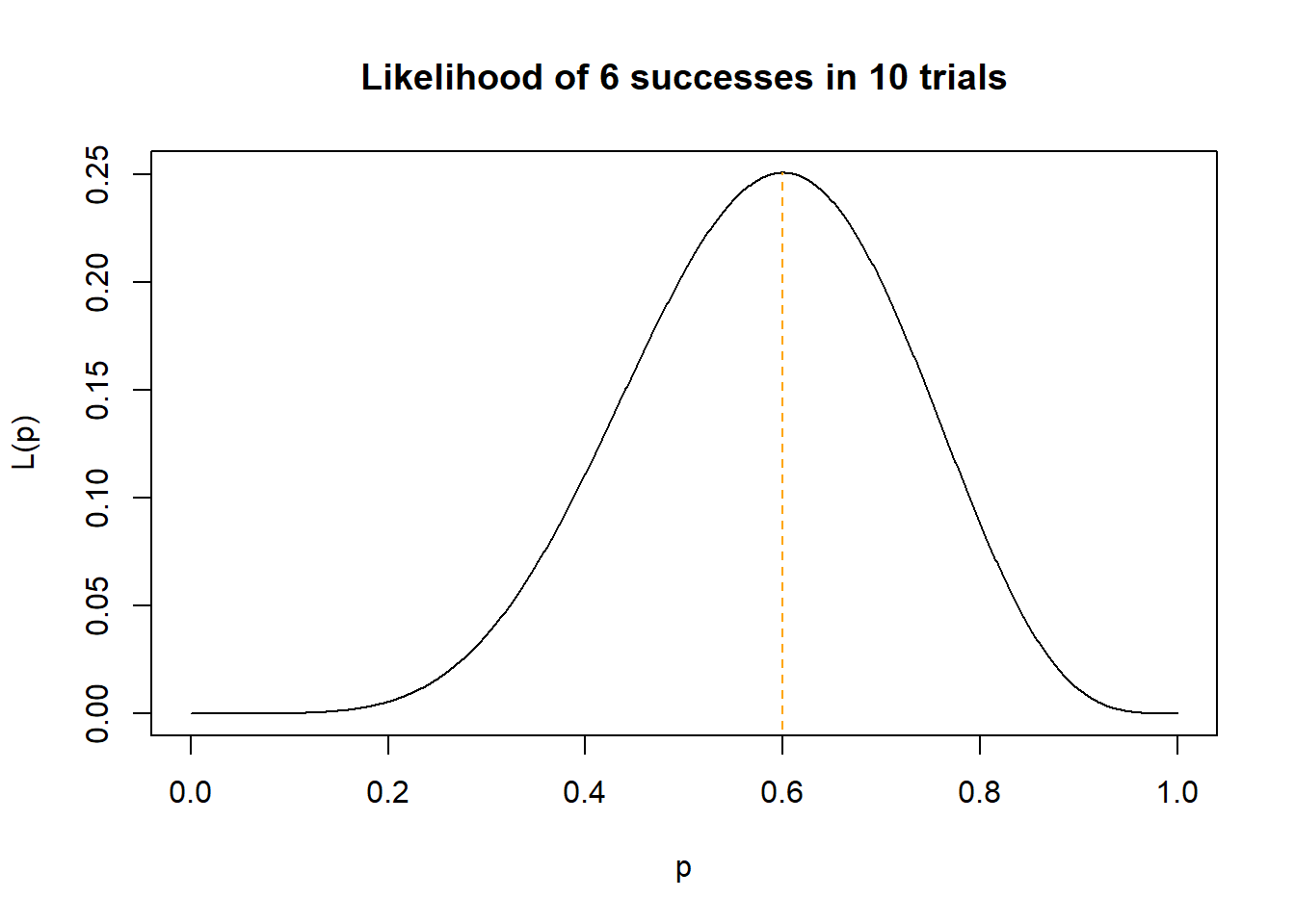
Continuing the previous part, use any software of your choice and plot the likelihood function. Based on your plot, what value appears to be the maximum likelihood estimate of \(p\) based on a sample with 6 heads in 10 flips? (You can do this just by zooming in on the plot.)
Continuing the previous part, carefully write the log-likelihood function.
Use calculus to find the maximum likelihood estimate of \(p\) based on observing 6 heads in 10 flips.
Now suppose you observe \(x\) heads in 10 flips. Carefully write the likelihood function.
Continuing the previous part, carefully write the log-likelihood function.
Use calculus to find a general expression for the maximum likelihood estimate of \(p\) based on observing \(x\) heads in 10 flips. (Your answer will be an expression involving \(x\).)
Solutions
Seems like the most natural estimator is \(X/n\), the sample proportion of H.
The observed sample proportion is \(6/10 = 0.6\), so the estimator \(X/n\) would estimate \(p\) to be 0.6 for this sample.
The “plus four” estimator basically appends 2 successes and 2 failures to the sample data and then computes the sample proportion based on the appended sample. (It is also a weighted average between the observe sample proportion \(X/n\) and 0.5.)
Based on the 6/10 sample, the plus four estimator estimates \(p\) to be \((6+2)/(10+4) = 8/14 = 0.571 = (10/14)(0.6) + (4/14)(0.5) = 0.571\).
We don’t know which of 0.6 and 0.571 is a better estimate because we don’t know what \(p\) is; that’s the reason why we’re trying to estimate it.
dbinom(6, 10, 0.6) = 0.251 = \(\binom{10}{6}(0.6)^6(1-0.6)^{10-6}\). If the probability that the coin lands on H is 0.6, then about 25.1 percent of sets of 10 flips would result in 6 H.
dbinom(6, 10, 0.571) = 0.186 = \(\binom{10}{6}(0.571)^6(1-0.571)^{10-6}\). If the probability that the coin lands on H is 0.571, then about 18.6 percent of sets of 10 flips would result in 6 H.
The likelihood of observing 6 H in 10 flips is greater if \(p = 0.6\) than if \(p = 0.571\), so if we’re trying to maximum the likelihood, we could pick 0.6 as our estimate of \(p\) based on the 6/10 sample.
When \(n=10\), \(X\) has a Binomial(10, \(p\)) distribution. The pmf is \(\binom{10}{x}p^x(1-p)^{10-x}.\) Plug in the observed data \(x=6\) and view the likelihood as a function of \(p\)\[
L(p) = \binom{10}{6}p^6(1-p)^{10-6}, \qquad 0<p<1
\]
See below. It seems like the overall maximum occurs at a value of 0.6.
Take logs \[
\ell(p) = \log L(p) = \log\left(\binom{10}{6}p^6(1-p)^{10-6}\right) = 6\log p + (10 - 6)\log(1-p) + \log\binom{10}{6}
\]
Differentiate the log-likelihood with respect to \(p\). (Don’t forget the chain rule for \(\log(1-p)\); the derivate of \(1-p\) on the inside is \(-1\).) \[
\ell'(p) = \frac{6}{p} + \frac{10 - 6}{1-p}(-1) + 0
\] Set \(\ell'(\hat{p}) = 0\) and solve to get \(\hat{p} = 0.6\). So the MLE of of \(p\) based on a sample of size 10 with 6 successes is 6/10 = 0.6, the observed sample proportion of success.
Replace 6 with a general \(x\)\[
L(p) = \binom{10}{x}p^x(1-p)^{10-x}, \qquad 0<p<1
\]
Continuing the previous part, carefully write the log-likelihood function. \[
\ell(p) = \log L(p) = \log\left(\binom{10}{x}p^x(1-p)^{10-x}\right) = x\log p + (10 - x)\log(1-p) + \log\binom{10}{x}
\]
Differentiate the log-likelihood with respect to \(p\). \(x\) is treated like a constant just like 6 above. (Don’t forget the chain rule for \(\log(1-p)\); the derivate of \(1-p\) on the inside is \(-1\).) \[
\ell'(p) = \frac{x}{p} + \frac{10 - x}{1-p}(-1) + 0
\] Set \(\ell'(\hat{p}) = 0\) and solve to get \(\hat{p} = x/10\). So the MLE of of \(p\) based on a sample of size 10 with \(x\) successes is \(x/10\), the observed sample proportion of success.
p =seq(0, 1, 0.001)plot(p, dbinom(6, 10, p), type ="l",xlab ="p",ylab ="L(p)",main ="Likelihood of 6 successes in 10 trials")segments(x0 =0.6, x1 =0.6, y0 =-1, y1 =dbinom(6, 10, 0.6), col ="orange", lty =2)
Problem 2
Suppose that times (minutes) between earthquakes (of any magnitude in a certain region) follow an Exponential distribution with rate parameter \(\lambda\). Let \(X_1, \ldots, X_n\) be a random sample of times (minutes) between earthquakes for \(n\) earthquakes. It can be shown that the MLE of \(\lambda\) is \(1/\bar{X}\).
Explain intuitively why \(1/\bar{X}\) is a reasonable estimator of \(\lambda\). Hint: it’s not just because it’s the MLE; think of properties of Exponential distributions.
Suppose the observed sample is: 20, 37, 13, 10, 25 minutes. Carefully write the likelihood function. (For a random sample from a continuous distribution, to find the likelihood function you plug each observed value into the pdf and then form the product.)
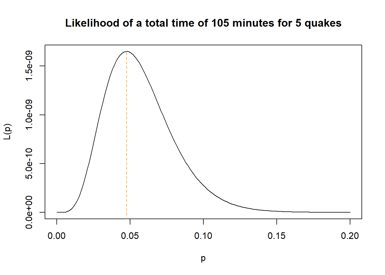
Use any software you want to carefully plot the likelihood function from the previous part. Then use your plot to verify that the MLE of \(\lambda\) based on this sample is \(1/\bar{x} = 5/105 = 0.0476\). (You can just zoom in on the plot.)
Write a clearly worded sentence reporting in context your estimate of \(\lambda\) from the previous part.
Solution
For Exponential, the population mean is the reciprocal of the rate, \(1/\lambda\). It seems reasonable to estimate the Exponential population mean \(1/\lambda\) with \(\bar{X}\), so it seems reasonable to estimate the rate \(\lambda\) with \(1/\bar{X}\).
Remember the Exponential pdf is \(\lambda e^{-\lambda x}\). There will be a factor in the likelihood for each observed \(x\) values. \[
L(\lambda) = \left(\lambda e^{-20\lambda }\right)\left(\lambda e^{-37\lambda }\right)\left(\lambda e^{-13\lambda }\right)\left(\lambda e^{-10\lambda }\right)\left(\lambda e^{-25\lambda }\right) = \lambda^5 e^{-\lambda(20 + 37 + 13 + 10 + 25 )}, \qquad \lambda >0
\]
See below. It looks like the MLE of \(\lambda\) based on this sample is \(1/\bar{x} = 5/105 = 0.0476\).
We estimate that earthquakes occur on average at rate 0.0476 earthquakes per minute (2.86 earthquakes per hour).
x =c(20, 37, 13, 10, 25)xbar =mean(x)lambda =seq(0, 0.2, 0.001)plot(lambda, lambda ^5*exp(-lambda *sum(x)), type ="l",xlab ="p",ylab ="L(p)",main ="Likelihood of a total time of 105 minutes for 5 quakes")segments(x0 =1/ xbar, x1 =1/ xbar, y0 =-1, y1 = (1/ xbar) ^5*exp(-(1/ xbar) *sum(x)), col ="orange", lty =2)