Assume a Poisson(\(\mu\)) model for the number of home runs hit (in total by both teams) in a MLB game. Let \(X_1, \ldots, X_n\) be a random sample of home run counts for \(n\) games.
Suppose we want to estimate \(\theta = \mu e^{-\mu}\), the probability that any single game has exactly 1 HR. Consider two estimators of \(\theta\)
\(\hat{\theta} = \bar{X} e^{-\bar{X}}\)
\(\hat{p} =\text{sample proportion of 1s} = \frac{\text{number of games in the sample with 1 HR}}{\text{sample size}}\)
Compute the value of \(\hat{\theta}\) based on the sample (3, 0, 1, 4, 0). Write a clearly worded sentence reporting in context this estimate of \(\theta\).
Compute the value of \(\hat{p}\) based on the sample (3, 0, 1, 4, 0). Write a clearly worded sentence reporting in context your estimate of \(\theta\).
Which of these two estimators is the MLE of \(\theta\) in this situation? Explain, without doing any calculations.
It can be shown that \(\hat{p}\) is an unbiased estimator of \(\theta\). Explain what this means.
Is \(\hat{\theta}\) an unbiased estimator of \(\theta\)? Explain. (You don’t have to derive anything; just apply a general principle.)
Suppose \(\mu = 2.3\) and \(n=5\). Explain in full detail how you would use simulation to approximate the bias of \(\hat{\theta}\).
Conduct the simulation from the previous part and plot the approximate of \(\hat{\theta}\) when \(\mu = 2.3\) and \(n = 5\).
Explain in full detail how you would use simulation to approximate the bias function of \(\hat{\theta}\) when \(n=5\).
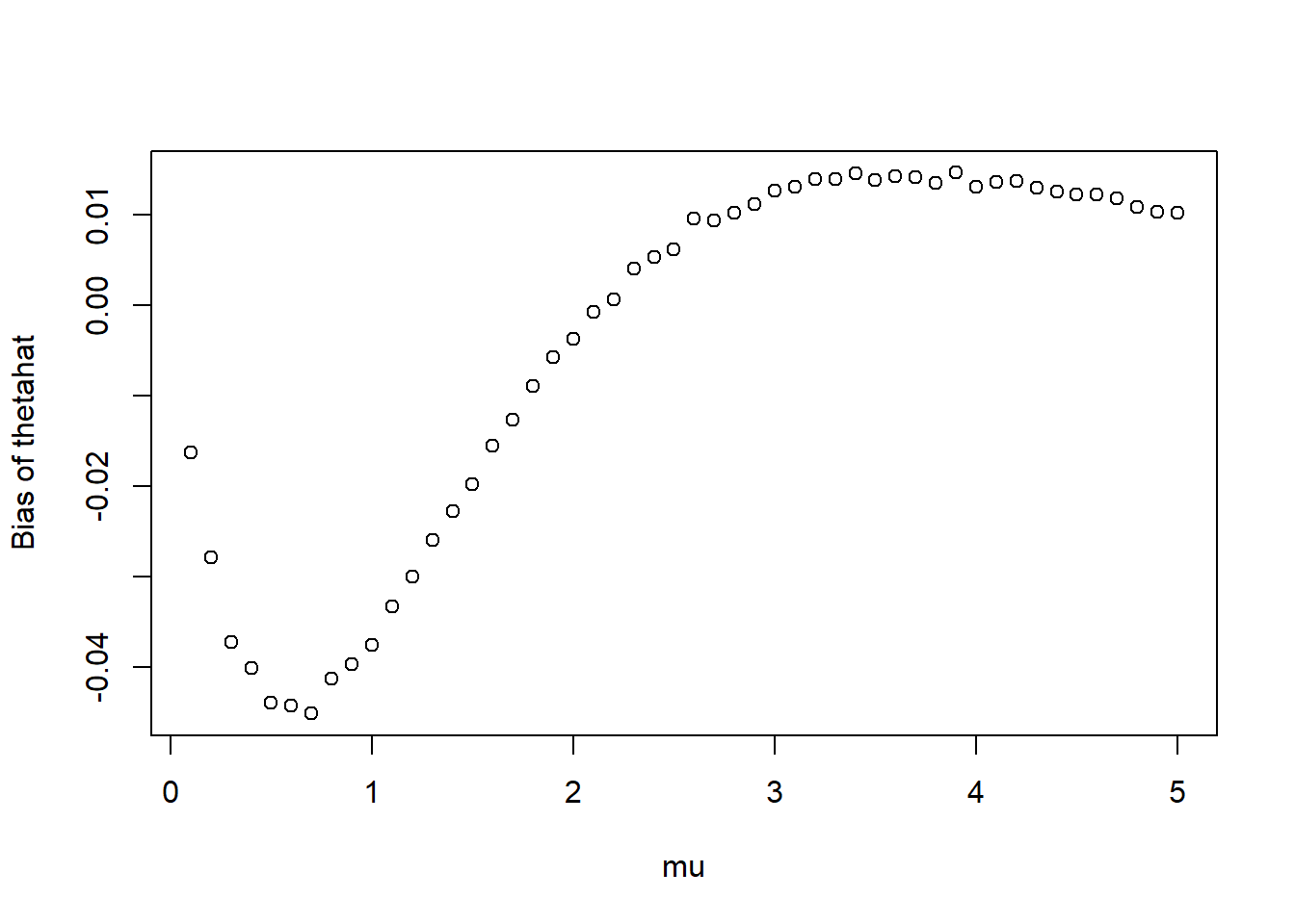
Conduct the simulation from the previous part and plot the approximate bias function when \(n=5\). For what values of \(\mu\) does \(\hat{\theta}\) tend to overestimate \(\mu\)? Underestimate? For what values of \(\mu\) is the bias the worst?
Solution
For the sample (3, 0, 1, 4, 0), the value of \(\bar{X}\) is 8/5 and the value of \(\hat{\theta}\) is \((8/5)e^{-8/5}=0.323\). Using this estimator, based on this sample we would estimate that 32.3 percent of baseball games have 1 home run.
For the sample (3, 0, 1, 4, 0) there is 1 game with 1 HR so \(\hat{p} = 1/5 = 0.2\). Using this estimator, based on this sample we would estimate that 20 percent of baseball games have 1 home run.
We know that the MLE of \(\mu\) for a Poisson distribution is \(\bar{X}\), so by the invariance principle of MLEs, \(\bar{X}e^{-\bar{X}}\) is the MLE of \(\mu e^{-\mu}\).
Over many samples, \(\hat{p}\) does not consistent over or under estimate \(\theta\).
No. \(\bar{X}\) is an unbiased estimator of \(\mu\) but nonlinear transformations do not preserve unbiasedness. \(\hat{\theta}\) is not unbiased estimator of \(\theta\). \[
\text{E}(\hat{\theta}) = \text{E}(\bar{X}e^{-\bar{X}})\neq \text{E}(\bar{X})e^{-\text{E}(\bar{X})} = \mu e^{-\mu} = \theta
\]
For \(\mu = 2.3\)
Simulate a sample of size \(n\) from a Poisson(2.3) distribution, say (3, 0, 1, 4, 0) for \(n=5\).
For the simulated sample compute the sample mean \(\bar{X}\) and the value of \(\hat{\theta} = \bar{X}e^{-\bar{X}}\), say 8/5 and \((8/5)e^{-8/5}=0.323\).
Repeat many times, simulating many samples of size \(n\) and many values of \(\hat{\theta}\) for the chosen \(\mu\).
Average the values of \(\hat{\theta}\) and subtract \(\theta=2.3 e^{-2.3}\) to approximate the bias when \(\mu = 2.3\).
See below.
We carry out the process in the previous part for many values of \(\mu\). Choose a grid of \(\mu\) values, say 0.01, 0.02, \(\ldots\), 10
Choose a value of \(\mu\) from the grid, say 2.3
Simulate a sample of size \(n\) from a Poisson(\(\mu\)) distribution, say (3, 0, 1, 4, 0) for \(n=5\).
For the simulated sample compute the sample mean \(\bar{X}\) and the value of \(\hat{\theta} = \bar{X}e^{-\bar{X}}\), say 8/5 and \((8/5)e^{-8/5}=0.323\).
Repeat many times, simulating many samples of size \(n\) and many values of \(\hat{\theta}\) for the chosen \(\mu\).
Average the values of \(\hat{\theta}\) and subtract \(\theta=\mu e^{-\mu}\) to approximate the bias for the chosen \(\mu\).
Repeat the above process for all the values of \(\mu\) in the grid and plot the approximate bias as a function of \(\mu\) to approximate the bias function.
See below.
Problem 2
Continuing Problem 2.
It can be shown that \(\text{Var}(\hat{p}) = \frac{\theta(1-\theta)}{n}\). Compute \(\text{Var}(\hat{p})\) when \(\mu = 2.3\) and \(n=5\). Then write a clearly worded sentence interpreting this value.
Suppose \(\mu = 2.3\) and \(n=5\). Explain in full detail how you would use simulation to approximate the variance of \(\hat{\theta}\).
Conduct the simulation from the previous part and approximate the variance of \(\hat{\theta}\) when \(\mu = 2.3\) and \(n=5\). Then write a clearly worded sentence interpreting this value.
Which estimator has smaller variance when \(\mu = 2.3\) (and \(n=5\))? Answer, but then explain why this information alone is not really useful.
Explain in full detail how you would use simulation to approximate the variance function of \(\hat{\theta}\) (if \(n=5\)).
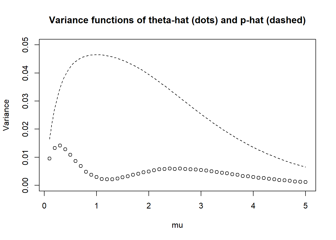
Conduct the simulation from the previous part and plot the approximate variance function. Compare to the variance function of \(\hat{p}\). Based on variability alone, which estimator is preferred?
Solution
When \(\mu = 2.3\), \(\theta = 2.3e^{-2.3} = 0.231\), so if \(n=5\)\[
\text{Var}_{\mu = 2.3}(\hat{p}) = \frac{0.231(1-0.231)}{5} = 0.035
\] This number measures the sample-to-sample variance of sample proportions of games with 1 HR over many samples of 5 games, assuming that \(\mu = 2.3\).
For \(\mu = 2.3\)
Simulate a sample of size \(n\) from a Poisson(2.3) distribution, say (3, 0, 1, 4, 0) for \(n=5\).
For the simulated sample compute the sample mean \(\bar{X}\) and the value of \(\hat{\theta} = \bar{X}e^{-\bar{X}}\), say 8/5 and \((8/5)e^{-8/5}=0.323\).
Repeat many times, simulating many samples of size \(n\) and many values of \(\hat{\theta}\) for the chosen \(\mu\).
Average the values of \(\hat{\theta}\), for each value of \(\hat{\theta}\) find its deviation from the average, and then average the squared deviations. This number approximates \(\text{Var}(\hat{\theta})\) when \(\mu = 2.3\)
See below. The value measures the sample-to-sample variance of values of \(\hat{\theta}\) (estimates of the probability that a game has 1 HR), assuming that \(\mu = 2.3\).
\(\hat{\theta}\) has smaller variance when \(\mu = 2.3\), but that by itself isn’t useful because we don’t know what \(\mu\) is.
We carry out the process in the previous part for many values of \(\mu\). Choose a grid of \(\mu\) values, say 0.01, 0.02, \(\ldots\), 10
Choose a value of \(\mu\) from the grid, say 2.3
Simulate a sample of size \(n\) from a Poisson(\(\mu\)) distribution, say (3, 0, 1, 4, 0) for \(n=5\).
For the simulated sample compute the sample mean \(\bar{X}\) and the value of \(\hat{\theta} = \bar{X}e^{-\bar{X}}\), say 8/5 and \((8/5)e^{-8/5}=0.323\).
Repeat many times, simulating many samples of size \(n\) and many values of \(\hat{\theta}\) for the chosen \(\mu\).
Average the values of \(\hat{\theta}\), for each value of \(\hat{\theta}\) find its deviation from the average, and then average the squared deviations. This number approximates \(\text{Var}(\hat{\theta})\) for the chosen \(\mu\)
Repeat the above process for all the values of \(\mu\) in the grid and plot the approximate bias as a function of \(\mu\) to approximate the bias function.
See below. Seems like \(\hat{\theta}\) has smaller variance regardless of \(\mu\).
Problem 3
Continuing Problems 2 and 3
Compute \(\text{MSE}(\hat{p})\) when \(\mu = 2.3\) and \(n=5\). (You can do the next part first if you want, but it helps to work with specific numbers first.)
Derive the MSE function of \(\hat{p}\). (Hint: see facts from previous parts.)
Suppose \(\mu = 2.3\) (and \(n=5\)). Explain in full detail how you would use simulation to approximate the MSE of \(\hat{\theta}\).
Conduct the simulation from the previous part and approximate the MSE of \(\hat{\theta}\) when \(\mu =2.3\) (and \(n=5\)).
Which estimator has smaller MSE when \(\mu = 2.3\) (and \(n=5\))? Answer, but then explain why this information alone is not really useful.
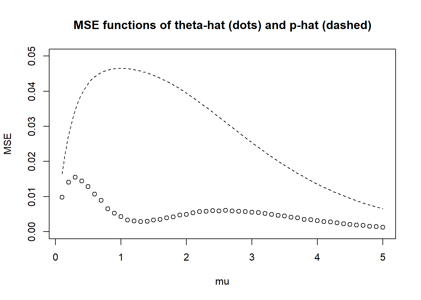
Conduct the simulation from the previous part and plot the approximate MSE function. Compare to the MSE function of \(\hat{p}\).
Compare the MSEs of the two estimators for \(n=5\) and a few other values of \(n\). Is there a clear preference between these two estimators? Discuss.
Solution
Since \(\hat{p}\) is unbiased, its MSE is just its variance.
Since \(\hat{p}\) is unbiased, its MSE function is just its variance function.
For \(\mu = 2.3\)
Simulate a sample of size \(n\) from a Poisson(2.3) distribution, say (3, 0, 1, 4, 0) for \(n=5\).
For the simulated sample compute the sample mean \(\bar{X}\) and the value of \(\hat{\theta} = \bar{X}e^{-\bar{X}}\), say 8/5 and \((8/5)e^{-8/5}=0.323\).
Repeat many times, simulating many samples of size \(n\) and many values of \(\hat{\theta}\) for the chosen \(\mu\).
For each value of \(\hat{\theta}\) subtract \(\theta=2.3 e^{-2.3}\) and square the difference, then average these squared differences to approximate the MSE when \(\mu = 2.3\).
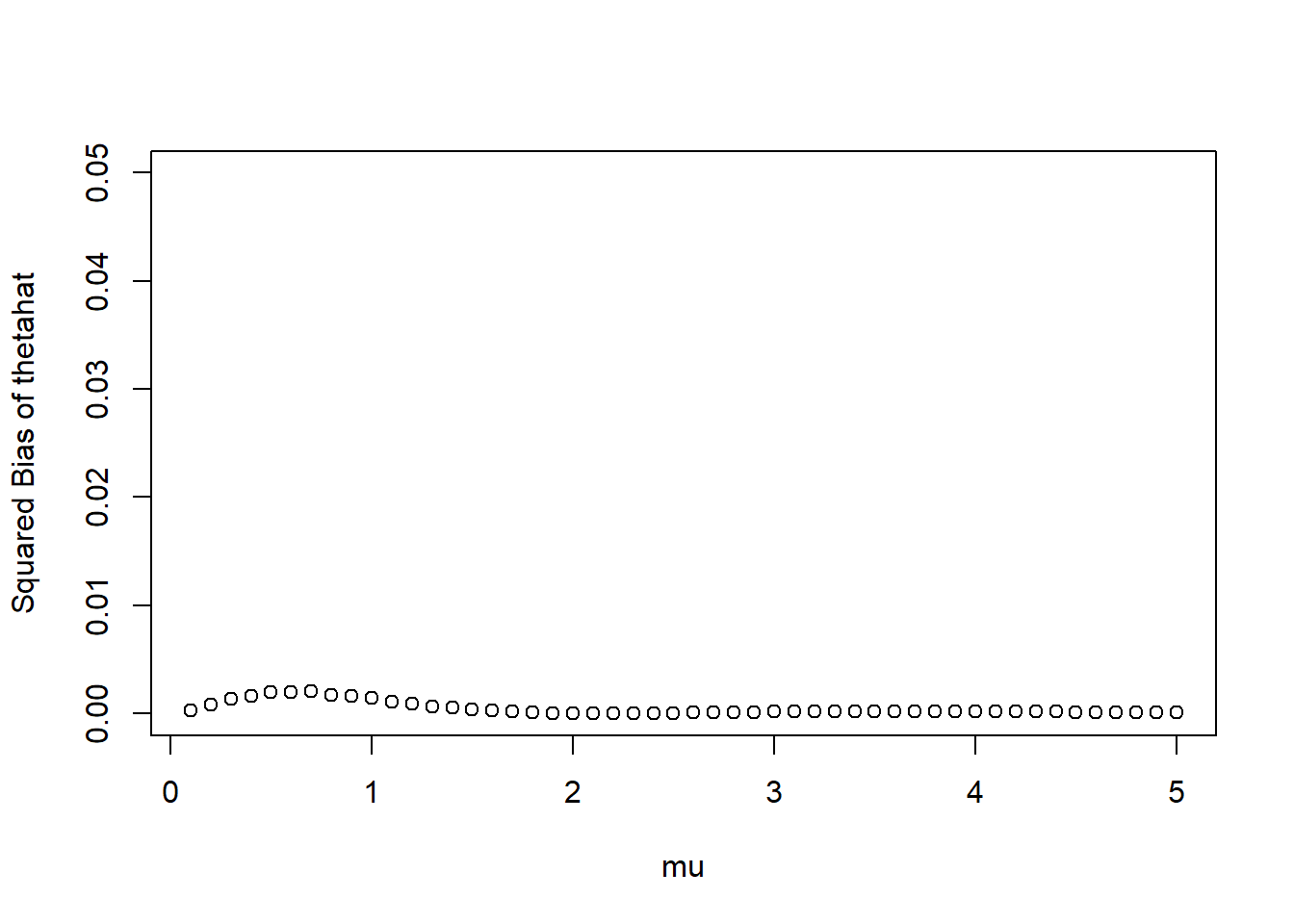
See below. The squared bias is fairly small compared to the variance, so the MSE is pretty close to the variance function.
\(\hat{\theta}\) has smaller MSE when \(\mu = 2.3\), but this isn’t really useful because we don’t know what \(\mu\) is.
See below.
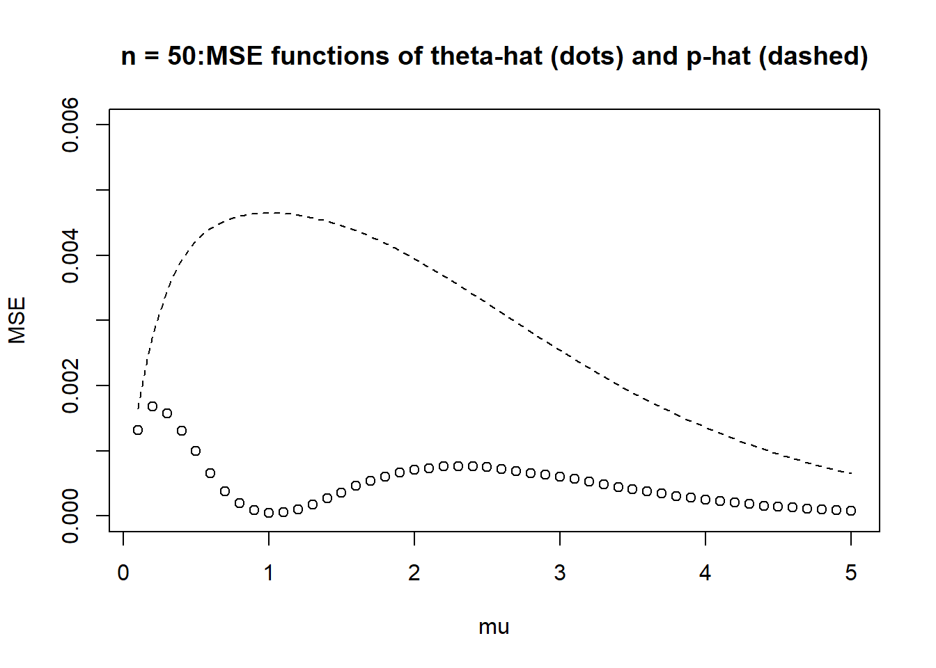
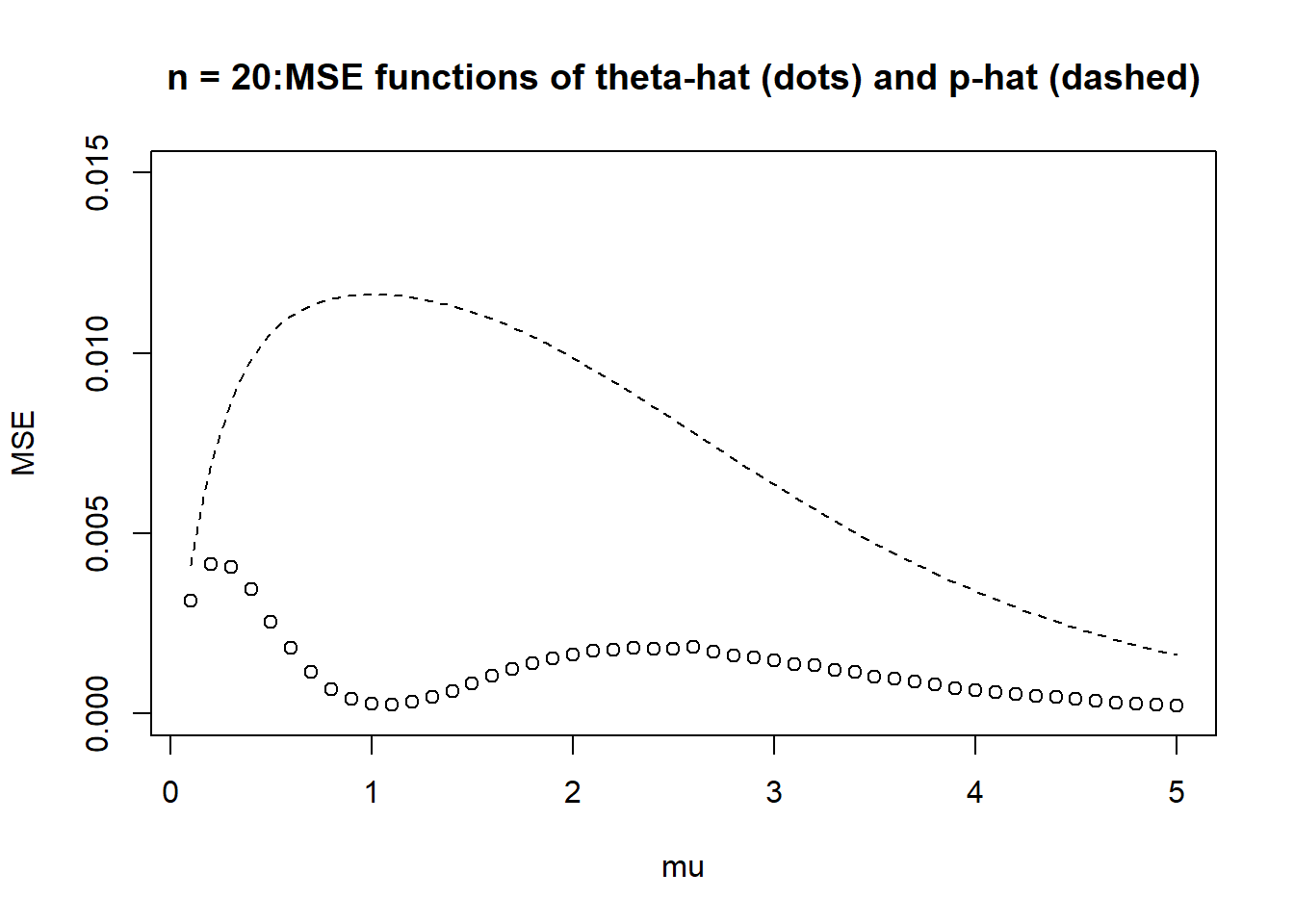
It seems that (at least for the values of \(n\) that we considered) \(\hat{\theta}\) has smaller MSE than \(\hat{p}\) for all \(\mu\). The sample proportion doesn’t use the fact that the population distribution is Poisson, and it treats each value as either 1 or not. \(\bar{X} e^{-\bar{X}}\) uses all the data and the fact that the population distribution is Poisson, so its better tuned to this problem.
Simulation
For mu = 2.3
n =5mu =2.3N_samples =10000theta_hats =vector(length = N_samples)for (i in1:N_samples) {# simulate a sample of size n from the Poisson(mu) population x =rpois(n, mu)# compute theta-hat theta_hats[i] =mean(x) *exp(-mean(x))}# Approximate the bias of theta-hat for this mumean(theta_hats) - mu *exp(-mu)
[1] 0.003518489
# Approximate the variance of theta-hat for this muvar(theta_hats)
[1] 0.005725971
# Approximate the MSE of theta-hat for this mumean((theta_hats - mu *exp(-mu)) ^2)
[1] 0.005737778
For all mu
n =5# grid of mu values: 0.1, 0.2, 0.3, ..., 4.9, 5mus =seq(0.1, 5, 0.1)N_samples =10000# initialize vectors that will record bias, var, mse as functions of mubias_thetahat =vector()var_thetahat =vector()mse_thetahat =vector()for (mu in mus) {# true value of theta for this mu theta = mu *exp(-mu)# for each mu simulate many samples and many values of sigma-hat^2 theta_hats =vector(length = N_samples)for (i in1:N_samples) {# simulate a sample of size n from the Poisson(mu) population x =rpois(n, mu)# compute theta-hat theta_hats[i] =mean(x) *exp(-mean(x)) }# Approximate bias of theta-hat for this mu and add to the list bias_thetahat =c(bias_thetahat, mean(theta_hats) - theta)# Approximate variance of sigma-hat^2 for this mu and add to the list var_thetahat =c(var_thetahat, var(theta_hats))# Approximate MSE of sigma-hat^2 for this mu and add to the list# Can just do bias^2 + var, but can also use definition of MSE mse_thetahat =c(mse_thetahat, mean((theta_hats - theta) ^2))}
Bias function
Any “wiggles” are due to natural simulation margin of error (can make these go away by simulating even more samples)
plot(mus, bias_thetahat,xlab ="mu",ylab ="Bias of thetahat")
Squared bias function
Any “wiggles” are due to natural simulation margin of error (can make these go away by simulating even more samples)
plot(mus, bias_thetahat ^2,xlab ="mu",ylab ="Squared Bias of thetahat",ylim =c(0, 0.05)) # set common y-axis scale
Variance function
Any “wiggles” are due to natural simulation margin of error (can make these go away by simulating even more samples)
plot(mus, var_thetahat,xlab ="mu",ylab ="Variance",ylim =c(0, 0.05), # set common y-axis scalemain ="Variance functions of theta-hat (dots) and p-hat (dashed)")curve(x *exp(-x) * (1- x *exp(-x)) / n, add =TRUE,lty =2)
MSE function
Any “wiggles” are due to natural simulation margin of error (can make these go away by simulating even more samples)
plot(mus, mse_thetahat,xlab ="mu",ylab ="MSE",ylim =c(0, 0.05), # set common y-axis scalemain ="MSE functions of theta-hat (dots) and p-hat (dashed)")curve(x *exp(-x) * (1- x *exp(-x)) / n, add =TRUE,lty =2)
Different n
n =50# grid of mu values: 0.1, 0.2, 0.3, ..., 4.9, 5mus =seq(0.1, 5, 0.1)N_samples =10000# initialize vectors that will record bias, var, mse as functions of mubias_thetahat =vector()var_thetahat =vector()mse_thetahat =vector()for (mu in mus) {# true value of theta for this mu theta = mu *exp(-mu)# for each mu simulate many samples and many values of sigma-hat^2 theta_hats =vector(length = N_samples)for (i in1:N_samples) {# simulate a sample of size n from the Poisson(mu) population x =rpois(n, mu)# compute theta-hat theta_hats[i] =mean(x) *exp(-mean(x)) }# Approximate bias of theta-hat for this mu and add to the list bias_thetahat =c(bias_thetahat, mean(theta_hats) - theta)# Approximate variance of sigma-hat^2 for this mu and add to the list var_thetahat =c(var_thetahat, var(theta_hats))# Approximate MSE of sigma-hat^2 for this mu and add to the list# Can just do bias^2 + var, but can also use definition of MSE mse_thetahat =c(mse_thetahat, mean((theta_hats - theta) ^2))}
plot(mus, mse_thetahat,xlab ="mu",ylab ="MSE",ylim =c(0, 0.006), # set common y-axis scalemain ="n = 50:MSE functions of theta-hat (dots) and p-hat (dashed)")curve(x *exp(-x) * (1- x *exp(-x)) / n, add =TRUE,lty =2)
n =20# grid of mu values: 0.1, 0.2, 0.3, ..., 4.9, 5mus =seq(0.1, 5, 0.1)N_samples =10000# initialize vectors that will record bias, var, mse as functions of mubias_thetahat =vector()var_thetahat =vector()mse_thetahat =vector()for (mu in mus) {# true value of theta for this mu theta = mu *exp(-mu)# for each mu simulate many samples and many values of sigma-hat^2 theta_hats =vector(length = N_samples)for (i in1:N_samples) {# simulate a sample of size n from the Poisson(mu) population x =rpois(n, mu)# compute theta-hat theta_hats[i] =mean(x) *exp(-mean(x)) }# Approximate bias of theta-hat for this mu and add to the list bias_thetahat =c(bias_thetahat, mean(theta_hats) - theta)# Approximate variance of sigma-hat^2 for this mu and add to the list var_thetahat =c(var_thetahat, var(theta_hats))# Approximate MSE of sigma-hat^2 for this mu and add to the list# Can just do bias^2 + var, but can also use definition of MSE mse_thetahat =c(mse_thetahat, mean((theta_hats - theta) ^2))}
plot(mus, mse_thetahat,xlab ="mu",ylab ="MSE",ylim =c(0, 0.015), # set common y-axis scalemain ="n = 20:MSE functions of theta-hat (dots) and p-hat (dashed)")curve(x *exp(-x) * (1- x *exp(-x)) / n, add =TRUE,lty =2)