CHAPTER 3 Estimation Procedures
Click for quick review
The Linear Model
\[ \underset{n\times1}{\textbf{Y}} = \underset{n\times (k+1)}{\textbf{X}}\underset{(k+1)\times1}{\boldsymbol{\beta}} + \underset{n\times 1}{\boldsymbol{\varepsilon}}\\\begin{bmatrix} Y_1 \\ Y_2 \\ \vdots\\ Y_n \end{bmatrix} =\begin{bmatrix} 1 & X_{11} & X_{12} & \cdots & X_{1k} \\ 1 & X_{21} & X_{12} & \cdots & X_{2k} \\ \vdots & \vdots & \vdots & \ddots & \vdots \\ 1 & X_{n1} & X_{n2} & \cdots & X_{nk} \end{bmatrix}\begin{bmatrix}\beta_0 \\ \beta_1 \\ \beta_2 \\ \vdots\\ \beta_k \end{bmatrix} + \begin{bmatrix} \varepsilon_1 \\ \varepsilon_2 \\ \vdots\\ \varepsilon_n\end{bmatrix} \]
where
- \(\textbf{Y}\) is the response vector.
- \(\textbf{X}\) is the design matrix.
- \(\boldsymbol{\beta}\) is the regression coefficients vector.
- \(\boldsymbol{\varepsilon}\) is the error term vector.
Assumptions
the expected value of the unknown quantity \(\varepsilon_i\) is 0 for every observation \(i\)
the variance of the errors term is the same for all observations
the error terms and observations are uncorrelated
the error terms follow a normal distribution
the independent variables are linearly independent from each other
Reasons for Having Assumptions
- to make sure that the parameters are estimable
- to make sure that the solution to the estimation problem is unique
- to aid in the interpretation of the model parameters
- to derive more important results that can be used for further analyses
GENERAL PROBLEM:
Given the following model, for observation \(i=1,...,n\) \[ Y_i=\beta_0+\beta_1X_{i1}+\beta_2 X_{i2}+\dots+\beta_kX_{ik}+\varepsilon_i \] or the matrix form \[ \textbf{Y} = \textbf{X}\boldsymbol{\beta}+\boldsymbol{\varepsilon} \] How do we estimate the \(\beta s\)?
There are several estimation procedures that can be used in linear models. The course will focus on least squares, but others are presented as well.
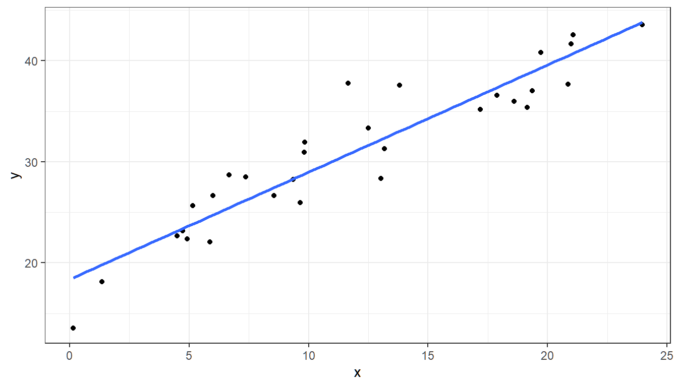
Figure 3.1: Scatterplot with fitted line
One criterion of the fitted line: have all points to be close to it. That is, we want to have small \(\varepsilon_i\)
3.1 Method of Least Squares
Objective function: Minimize \(\sum_{i=1}^n\varepsilon_i^2\) or \(\boldsymbol{\varepsilon}'\boldsymbol{\varepsilon}\) , the inner product of the error term vector.
In simple linear regression \(y_i=\beta_0 +\beta x_i+\varepsilon_i\), the estimator for \(\beta_0\) and \(\beta\) can be derived as follows:
\[
\hat{\beta_0}=\underset{\beta_0}{\arg \min}\sum_{i=1}^n \varepsilon_i^2 \quad
\hat{\beta}=\underset{\beta}{\arg \min}\sum_{i=1}^n \varepsilon_i^2
\]
Full solution
GOAL: Find value of \(\beta_0\) and \(\beta\) that minimizes \(\sum_{i=1}^n\varepsilon_i^2\), which are the solutions to the equations \[ \frac{d}{d\beta_0}\sum_{i=1}^n\varepsilon_i^2=0\quad\text{and}\quad\frac{d}{d\beta}\sum_{i=1}^n\varepsilon_i^2=0 \]
For the Intercept
\[\begin{align} \frac{d}{d\beta_0}\sum_{i=1}^n\varepsilon_i^2 &= \frac{d}{d\beta_0}\sum_{i=1}^n(y_i-\beta_0-\beta x_i)^2 \\ &= -2\sum_{i=1}^n(y_i-\beta_0-\beta x_i) \end{align}\]
Now, equate to \(0\) and solve for \(\hat{\beta_0}\)
\[\begin{align} 0&=-2\sum_{i=1}^n(y_i-\hat{\beta_0}-\hat{\beta} x_i)\\ 0&=\sum_{i=1}^ny_i - n\hat{\beta_0}-\hat{\beta} \sum_{i=1}^nx_i\\ n\hat{\beta_0} &= \sum_{i=1}^ny_i -\hat{\beta} \sum_{i=1}^nx_i \\ \hat{\beta_0} &= \bar{y} -\hat{\beta} \bar{x} \end{align}\]
For the Slope
Since there is already an estimate for \(\beta_0\), we can already plug it in the equation before solving for \(\hat{\beta}\).
\[\begin{align} \frac{d}{d\beta}\sum_{i=1}^n\varepsilon^2 &= \frac{d}{d\beta}\sum_{i=1}^n[y_i-\hat{\beta_0}-\beta x_i]^2 \\ &= \frac{d}{d\beta}\sum_{i=1}^n[y_i-(\bar{y}-\beta\bar{x})-\beta x_i]^2 \\ &= \frac{d}{d\beta}\sum_{i=1}^n[(y_i-\bar{y})-\beta( x_i-\bar{x})]^2 \\ &= -2\sum_{i=1}^n\left\{[(y_i-\bar{y})-\beta( x_i-\bar{x})]( x_i-\bar{x})\right\} \\ &= -2\sum_{i=1}^n[(y_i-\bar{y})( x_i-\bar{x})-\beta( x_i-\bar{x})( x_i-\bar{x})] \end{align}\]
Equating to \(0\) to solve for \(\hat{\beta_0}\)
\[\begin{align} 0 &= -2\sum_{i=1}^n[(y_i-\bar{y})( x_i-\bar{x})-\hat{\beta}( x_i-\bar{x})( x_i-\bar{x})] \\ 0 &= \sum_{i=1}^n[(y_i-\bar{y})( x_i-\bar{x})]- \hat{\beta}\sum_{i=1}^n( x_i-\bar{x})^2 \\ \hat{\beta}&= \frac{\sum_{i=1}^n[(y_i-\bar{y})( x_i-\bar{x})]}{\sum_{i=1}^n( x_i-\bar{x})^2} \end{align}\]
Therefore, we have \(\hat{\beta_0} = \bar{y} -\hat{\beta} \bar{x}\) and \(\hat{\beta} = \frac{\sum_{i=1}^n(y_i-\bar{y})(x_i-\bar{x})}{\sum_{i=1}^n( x_i-\bar{x})^2}\) \(\blacksquare\)
How do we generalize this for the multiple linear regression?
The Normal Equations
Definition 3.1 The normal equation is a closed-form solution used to find an estimated value of the parameter that minimizes an objective function.
In the least squares method, the objective function (or the cost function) is \(\boldsymbol{\varepsilon}'\boldsymbol{\varepsilon}=(\textbf{Y}-\textbf{X}\boldsymbol{\beta})'(\textbf{Y}-\textbf{X}\boldsymbol{\beta})\).
If we minimize this with respect to the parameters \(\beta_j\), we will obtain the normal equations \(\frac{\partial\boldsymbol{\varepsilon}'\boldsymbol{\varepsilon}}{\partial\beta_j} = 0, \quad j =0,...,k\). Expanding this, we have the following normal equations:
In \((k+1)\) equations form : \(\frac{\partial\sum_{i=1}^n\varepsilon_i^2}{\partial\beta_j} = 0, \quad j =0,...,k\)
\[\begin{align}1st :&\quad \hat\beta_0n +\hat\beta_1\sum X_{i1} + \hat\beta_2\sum X_{i2} + \cdots + \hat\beta_k\sum X_{ik}&=\quad&\sum Y_i \\2nd :&\quad \hat\beta_0\sum X_{i1} + \hat\beta_1\sum X_{i1}^2 + \hat\beta_2\sum X_{i1}X_{i2} + \cdots + \hat\beta_k\sum X_{i1}X_{ik} &=\quad& \sum X_{i1} Y_i \\ \vdots\quad & &&\quad\vdots \\ (k+1)th :&\quad \hat\beta_0\sum X_{ik} + \hat\beta_1\sum X_{i1} X_{ik} + \hat\beta_2\sum X_{i2}X_{ik} + \cdots + \hat\beta_k\sum X_{ik}^2 &=\quad& \sum X_{ik} Y_i\end{align}\]
In matrix form: \(\frac{\partial\boldsymbol{\varepsilon}'\boldsymbol{\varepsilon}}{\partial{\boldsymbol{\beta}}} = \textbf{0}\)
\[ \textbf{X}'\textbf{X}\hat{\boldsymbol{\beta}} = \textbf{X}'\textbf{Y} \]
\[ \begin{bmatrix}n & \sum X_{i1} & \sum X_{i2} & \cdots & \sum X_{ik} \\\sum X_{i1} & \sum X_{i1}^2 & \sum X_{i1}X_{i2} & \cdots & \sum X_{i1}X_{ik} \\\vdots & \vdots & \vdots & \ddots & \vdots \\\sum X_{ik} & \sum X_{i1} X_{ik} & \sum X_{i2}X_{ik} & \cdots & \sum X_{ik}^2 \\\end{bmatrix}\begin{bmatrix} \hat{\beta_0}\\ \hat\beta_1\\ \hat\beta_2\\ \vdots \\ \hat\beta_k\end{bmatrix}= \begin{bmatrix} \sum Y_i \\ \sum X_{i1} Y_i \\ \vdots\\ \sum X_{ik} Y_i\end{bmatrix} \]
The solution to these equations is unique, and will be the ordinary least squares estimator for \(\boldsymbol{\beta}\).
All of these normal equations are unconditionally true under method of least squares.
The OLS Estimator
Theorem 3.1 (Ordinary Least Squares Estimator)
\[ \boldsymbol{\hat{\beta}}=(\textbf{X}'\textbf{X})^{-1}(\textbf{X}'\textbf{Y}) \]
Remarks:
\((\textbf{X}'\textbf{X})^{−1}\) exists when \(\textbf{X}\) is of full column rank.
This implies that the independent variables should be independent from each other.
Furthermore, if \(n < p\), then \(\textbf{X}\) cannot be full column rank. Therefore, there should be more observations than the number of regressors.
Since the estimator \(\hat{\boldsymbol{\beta}}\) is a random vector, we also want to explore its mean and variance.
Theorem 3.2 The OLS estimator \(\hat{\boldsymbol\beta}\) is an unbiased estimator for \(\boldsymbol{\beta}\)
Theorem 3.3 The variance-covariance matrix of \(\hat{\boldsymbol{\beta}}\) is given by \(\sigma^2(\textbf{X}'\textbf{X})^{-1}\)
Remark: \(Var(\hat{\beta}_j)\) is the \((j+1)^{th}\) diagonal element of \(\sigma^2(\textbf{X}'\textbf{X})^{-1}\)
More properties regarding the method of least squares will be discussed in Section 4.5 , where we also explain that the OLS estimator for \(\boldsymbol{\beta}\) is also the BLUE, MLE, and UMVUE for \(\boldsymbol{\beta}\)
Q: What does it mean when the variance of an estimator \(\hat{\beta}_j\) is large?
Exercises
Exercise 3.1 Prove Theorem 3.1
Assume that \((\textbf{X}'\textbf{X})^{-1}\) exists.
Hints
- Minimize \(\boldsymbol{\varepsilon}'\boldsymbol{\varepsilon}\) with respect to \(\boldsymbol{\beta}\).
- Note that \(\boldsymbol{\varepsilon}=\textbf{Y}-\textbf{X}\boldsymbol{\beta}\).
- Recall matrix calculus.
- You will obtain the normal equations, then solve for \(\boldsymbol{\beta}\).
Exercise 3.2 Prove Theorem 3.2
Hint
- Show \(E(\hat{\boldsymbol{\beta}})=\boldsymbol{\beta}\)
Exercise 3.3 Prove Theorem 3.3
Hint
- Show \(Var(\hat{\boldsymbol{\beta}})= \sigma^2(\textbf{X}'\textbf{X})^{-1}\)
The following exercises will help us understand some requirements before obtaining the estimate \(\hat{\boldsymbol{\beta}}\)
Exercise 3.4 Let \(\textbf{X}\) be the \(n\times p\) design matrix. Prove that if \(\textbf{X}\) has linearly dependent columns, then \(\textbf{X}'\textbf{X}\) is not invertible
Hints
The following should be part of your proof. Do not forget to cite reasons.
- highest possible rank of \(\textbf{X}\)
- highest possible rank of \(\textbf{X}'\textbf{X}\)
- order of \(\textbf{X}'\textbf{X}\)
- determinant of \(\textbf{X}'\textbf{X}\)
Exercise 3.5 Prove that if \(n < p\), then \(\textbf{X}'\textbf{X}\) is not invertible.
Hints
Almost same hints as previous exercise.
3.2 Other Estimation Methods
As mentioned, we will focus on the least squares estimation in this course. The following are just quick introduction of other methods in estimating the coefficients or the equation that predicts \(Y\)
Method of Least Absolute Deviations
Objective function: Minimize \(\sum_{i=1}^n|\varepsilon_i|\)
- Solution is quantile regression model.
- Solution is robust to extreme observations. The method places less emphasis on outlying observations than does the method of least squares.
- This method is one of a variety of robust methods that have the property of being insensitive to both outlying data values and inadequacies of the model employed.
- The solution may not be unique.
Backfitting Method
Assuming an additive model \[ Y_i=\beta_0+ \beta_1X_{i1}+\beta_2X_{i2}+\cdots+\beta_kX_{ik}+\varepsilon_i \] with constraints \(\sum_{i=1}^n\beta_jX_{ij}=0\) for $j=1,…,k$ and \(\quad \beta_0=\frac{1}{n\sum_{i=1}^nY_i}\)
Fit the coefficient of the most important variable.
Compute for residuals: \(Y_1 = Y − \hat{\beta}_1 X_1\)
Fit the coefficient for the next important variable.
Compute for residuals: \(Y_2 = Y_1 − \hat{\beta}_2 X_2\)
Continue until last coefficient is computed.
Gradient Descent
Gradient Descent is an optimization algorithm for finding a local minimum of a differentiable function. This is one of the first algorithms that you will encounter if you will study machine learning.

- Initialize the parameters of the model randomly
- Compute the gradient of the cost function with respect to each parameter. It involves making partial differentiation of cost function with respect to the parameters.
- Update the parameters of the model by taking steps in the opposite direction of the model. Choose a hyperparameter learning rate which is denoted by alpha. It helps in deciding the step size of the gradient.
- Repeat steps 2 and 3 iteratively to get the best parameter for the defined model.
If the cost function is the sum of squares of errors, then OLS is better.
But if the cost function has no closed form solution, then gradient descent may become useful.
Source: https://www.geeksforgeeks.org/gradient-descent-in-linear-regression/
Nonparametric Regression
Fit the model \(Y = f (X_1, X2, \cdots , X_k ) + \varepsilon_i\) where the function \(f\) is has no parameters.
It is the unknown function \(f\) being estimated, not just the parameters as what we do in parametric fitting.
Some examples:
- Kernel Estimation
- Projection Pursuit
- Spline Smoothing
- Wavelets Fitting
- Iterative Backfitting
Example(Anscombe dataset): predict per capita income based on budget for education of a state.
| education | income | young | urban | |
|---|---|---|---|---|
| ME | 189 | 2824 | 350.7 | 508 |
| NH | 169 | 3259 | 345.9 | 564 |
| VT | 230 | 3072 | 348.5 | 322 |
| MA | 168 | 3835 | 335.3 | 846 |
| RI | 180 | 3549 | 327.1 | 871 |
| CT | 193 | 4256 | 341.0 | 774 |
| NY | 261 | 4151 | 326.2 | 856 |
| NJ | 214 | 3954 | 333.5 | 889 |
| PA | 201 | 3419 | 326.2 | 715 |
| OH | 172 | 3509 | 354.5 | 753 |
| IN | 194 | 3412 | 359.3 | 649 |
| IL | 189 | 3981 | 348.9 | 830 |
| MI | 233 | 3675 | 369.2 | 738 |
| WI | 209 | 3363 | 360.7 | 659 |
| MN | 262 | 3341 | 365.4 | 664 |
| IO | 234 | 3265 | 343.8 | 572 |
| MO | 177 | 3257 | 336.1 | 701 |
| ND | 177 | 2730 | 369.1 | 443 |
| SD | 187 | 2876 | 368.7 | 446 |
| NE | 148 | 3239 | 349.9 | 615 |
| KA | 196 | 3303 | 339.9 | 661 |
| DE | 248 | 3795 | 375.9 | 722 |
| MD | 247 | 3742 | 364.1 | 766 |
| DC | 246 | 4425 | 352.1 | 1000 |
| VA | 180 | 3068 | 353.0 | 631 |
| WV | 149 | 2470 | 328.8 | 390 |
| NC | 155 | 2664 | 354.1 | 450 |
| SC | 149 | 2380 | 376.7 | 476 |
| GA | 156 | 2781 | 370.6 | 603 |
| FL | 191 | 3191 | 336.0 | 805 |
| KY | 140 | 2645 | 349.3 | 523 |
| TN | 137 | 2579 | 342.8 | 588 |
| AL | 112 | 2337 | 362.2 | 584 |
| MS | 130 | 2081 | 385.2 | 445 |
| AR | 134 | 2322 | 351.9 | 500 |
| LA | 162 | 2634 | 389.6 | 661 |
| OK | 135 | 2880 | 329.8 | 680 |
| TX | 155 | 3029 | 369.4 | 797 |
| MT | 238 | 2942 | 368.9 | 534 |
| ID | 170 | 2668 | 367.7 | 541 |
| WY | 238 | 3190 | 365.6 | 605 |
| CO | 192 | 3340 | 358.1 | 785 |
| NM | 227 | 2651 | 421.5 | 698 |
| AZ | 207 | 3027 | 387.5 | 796 |
| UT | 201 | 2790 | 412.4 | 804 |
| NV | 225 | 3957 | 385.1 | 809 |
| WA | 215 | 3688 | 341.3 | 726 |
| OR | 233 | 3317 | 332.7 | 671 |
| CA | 273 | 3968 | 348.4 | 909 |
| AK | 372 | 4146 | 439.7 | 484 |
| HI | 212 | 3513 | 382.9 | 831 |
##
## Call:
## lm(formula = income ~ education, data = Anscombe)
##
## Coefficients:
## (Intercept)    education
##    1645.383        8.048
# Least Absolute Deviation (Quantile Regression)
library(quantreg)
rq(income ~ education, data = Anscombe)## Call:
## rq(formula = income ~ education, data = Anscombe)
##
## Coefficients:
## (Intercept) education
## 1209.67290 10.25234
##
## Degrees of freedom: 51 total; 49 residual3.3 Interpretation of the Coefficients
In general, ceteris paribus(all things being the same)
\(\hat{\beta_j}\) = change in the estimated mean of \(Y\) per unit change in variable \(X_j\) holding other independent variables constant.
\(\hat{\beta_0}\) = value of the estimated mean of \(Y\) when all independent variables are set to 0.
We don’t always interpret the intercept, but why include it in the estimation?
Figure 3.2: Fitted line if estimated intercept is forced to be 0
- Intercept is only interpretable if a value of 0 is logical for all independent variables included in the model.
- Regardless of its interpretability, we still include it in the estimation. That is why in the design matrix \(\textbf{X}\), the first column is a vector of \(1\)s
- If we force to have an intercept of equal to 0, then the fitted line is the line that passes through the center of the points and the origin.
Caution on the Interpretation of the Coefficients
- Coefficients are partial. Assume that other effects are held constant.
- Validity of interpretation depends on whether the assumption of uncorrelatedness among the \(X_j\)s holds
- Affected by the range of \(X\) used in estimation
Example:
Suppose that we are statistical consultants hired by a client to provide advice on how to improve sales of a particular product. The advertising data set (from ISLR) consists of the sales of that product in 200 different markets, along with advertising budgets for the product in each of those markets for three different media: TV, radio, and newspaper.
| id | tv | radio | newspaper | sales |
|---|---|---|---|---|
| 1 | 230.1 | 37.8 | 69.2 | 22.1 |
| 2 | 44.5 | 39.3 | 45.1 | 10.4 |
| 3 | 17.2 | 45.9 | 69.3 | 9.3 |
| 4 | 151.5 | 41.3 | 58.5 | 18.5 |
| 5 | 180.8 | 10.8 | 58.4 | 12.9 |
| 6 | 8.7 | 48.9 | 75.0 | 7.2 |
| 7 | 57.5 | 32.8 | 23.5 | 11.8 |
| 8 | 120.2 | 19.6 | 11.6 | 13.2 |
| 9 | 8.6 | 2.1 | 1.0 | 4.8 |
| 10 | 199.8 | 2.6 | 21.2 | 10.6 |
| 11 | 66.1 | 5.8 | 24.2 | 8.6 |
| 12 | 214.7 | 24.0 | 4.0 | 17.4 |
| 13 | 23.8 | 35.1 | 65.9 | 9.2 |
| 14 | 97.5 | 7.6 | 7.2 | 9.7 |
| 15 | 204.1 | 32.9 | 46.0 | 19.0 |
| 16 | 195.4 | 47.7 | 52.9 | 22.4 |
| 17 | 67.8 | 36.6 | 114.0 | 12.5 |
| 18 | 281.4 | 39.6 | 55.8 | 24.4 |
| 19 | 69.2 | 20.5 | 18.3 | 11.3 |
| 20 | 147.3 | 23.9 | 19.1 | 14.6 |
| 21 | 218.4 | 27.7 | 53.4 | 18.0 |
| 22 | 237.4 | 5.1 | 23.5 | 12.5 |
| 23 | 13.2 | 15.9 | 49.6 | 5.6 |
| 24 | 228.3 | 16.9 | 26.2 | 15.5 |
| 25 | 62.3 | 12.6 | 18.3 | 9.7 |
| 26 | 262.9 | 3.5 | 19.5 | 12.0 |
| 27 | 142.9 | 29.3 | 12.6 | 15.0 |
| 28 | 240.1 | 16.7 | 22.9 | 15.9 |
| 29 | 248.8 | 27.1 | 22.9 | 18.9 |
| 30 | 70.6 | 16.0 | 40.8 | 10.5 |
| 31 | 292.9 | 28.3 | 43.2 | 21.4 |
| 32 | 112.9 | 17.4 | 38.6 | 11.9 |
| 33 | 97.2 | 1.5 | 30.0 | 9.6 |
| 34 | 265.6 | 20.0 | 0.3 | 17.4 |
| 35 | 95.7 | 1.4 | 7.4 | 9.5 |
| 36 | 290.7 | 4.1 | 8.5 | 12.8 |
| 37 | 266.9 | 43.8 | 5.0 | 25.4 |
| 38 | 74.7 | 49.4 | 45.7 | 14.7 |
| 39 | 43.1 | 26.7 | 35.1 | 10.1 |
| 40 | 228.0 | 37.7 | 32.0 | 21.5 |
| 41 | 202.5 | 22.3 | 31.6 | 16.6 |
| 42 | 177.0 | 33.4 | 38.7 | 17.1 |
| 43 | 293.6 | 27.7 | 1.8 | 20.7 |
| 44 | 206.9 | 8.4 | 26.4 | 12.9 |
| 45 | 25.1 | 25.7 | 43.3 | 8.5 |
| 46 | 175.1 | 22.5 | 31.5 | 14.9 |
| 47 | 89.7 | 9.9 | 35.7 | 10.6 |
| 48 | 239.9 | 41.5 | 18.5 | 23.2 |
| 49 | 227.2 | 15.8 | 49.9 | 14.8 |
| 50 | 66.9 | 11.7 | 36.8 | 9.7 |
| 51 | 199.8 | 3.1 | 34.6 | 11.4 |
| 52 | 100.4 | 9.6 | 3.6 | 10.7 |
| 53 | 216.4 | 41.7 | 39.6 | 22.6 |
| 54 | 182.6 | 46.2 | 58.7 | 21.2 |
| 55 | 262.7 | 28.8 | 15.9 | 20.2 |
| 56 | 198.9 | 49.4 | 60.0 | 23.7 |
| 57 | 7.3 | 28.1 | 41.4 | 5.5 |
| 58 | 136.2 | 19.2 | 16.6 | 13.2 |
| 59 | 210.8 | 49.6 | 37.7 | 23.8 |
| 60 | 210.7 | 29.5 | 9.3 | 18.4 |
| 61 | 53.5 | 2.0 | 21.4 | 8.1 |
| 62 | 261.3 | 42.7 | 54.7 | 24.2 |
| 63 | 239.3 | 15.5 | 27.3 | 15.7 |
| 64 | 102.7 | 29.6 | 8.4 | 14.0 |
| 65 | 131.1 | 42.8 | 28.9 | 18.0 |
| 66 | 69.0 | 9.3 | 0.9 | 9.3 |
| 67 | 31.5 | 24.6 | 2.2 | 9.5 |
| 68 | 139.3 | 14.5 | 10.2 | 13.4 |
| 69 | 237.4 | 27.5 | 11.0 | 18.9 |
| 70 | 216.8 | 43.9 | 27.2 | 22.3 |
| 71 | 199.1 | 30.6 | 38.7 | 18.3 |
| 72 | 109.8 | 14.3 | 31.7 | 12.4 |
| 73 | 26.8 | 33.0 | 19.3 | 8.8 |
| 74 | 129.4 | 5.7 | 31.3 | 11.0 |
| 75 | 213.4 | 24.6 | 13.1 | 17.0 |
| 76 | 16.9 | 43.7 | 89.4 | 8.7 |
| 77 | 27.5 | 1.6 | 20.7 | 6.9 |
| 78 | 120.5 | 28.5 | 14.2 | 14.2 |
| 79 | 5.4 | 29.9 | 9.4 | 5.3 |
| 80 | 116.0 | 7.7 | 23.1 | 11.0 |
| 81 | 76.4 | 26.7 | 22.3 | 11.8 |
| 82 | 239.8 | 4.1 | 36.9 | 12.3 |
| 83 | 75.3 | 20.3 | 32.5 | 11.3 |
| 84 | 68.4 | 44.5 | 35.6 | 13.6 |
| 85 | 213.5 | 43.0 | 33.8 | 21.7 |
| 86 | 193.2 | 18.4 | 65.7 | 15.2 |
| 87 | 76.3 | 27.5 | 16.0 | 12.0 |
| 88 | 110.7 | 40.6 | 63.2 | 16.0 |
| 89 | 88.3 | 25.5 | 73.4 | 12.9 |
| 90 | 109.8 | 47.8 | 51.4 | 16.7 |
| 91 | 134.3 | 4.9 | 9.3 | 11.2 |
| 92 | 28.6 | 1.5 | 33.0 | 7.3 |
| 93 | 217.7 | 33.5 | 59.0 | 19.4 |
| 94 | 250.9 | 36.5 | 72.3 | 22.2 |
| 95 | 107.4 | 14.0 | 10.9 | 11.5 |
| 96 | 163.3 | 31.6 | 52.9 | 16.9 |
| 97 | 197.6 | 3.5 | 5.9 | 11.7 |
| 98 | 184.9 | 21.0 | 22.0 | 15.5 |
| 99 | 289.7 | 42.3 | 51.2 | 25.4 |
| 100 | 135.2 | 41.7 | 45.9 | 17.2 |
| 101 | 222.4 | 4.3 | 49.8 | 11.7 |
| 102 | 296.4 | 36.3 | 100.9 | 23.8 |
| 103 | 280.2 | 10.1 | 21.4 | 14.8 |
| 104 | 187.9 | 17.2 | 17.9 | 14.7 |
| 105 | 238.2 | 34.3 | 5.3 | 20.7 |
| 106 | 137.9 | 46.4 | 59.0 | 19.2 |
| 107 | 25.0 | 11.0 | 29.7 | 7.2 |
| 108 | 90.4 | 0.3 | 23.2 | 8.7 |
| 109 | 13.1 | 0.4 | 25.6 | 5.3 |
| 110 | 255.4 | 26.9 | 5.5 | 19.8 |
| 111 | 225.8 | 8.2 | 56.5 | 13.4 |
| 112 | 241.7 | 38.0 | 23.2 | 21.8 |
| 113 | 175.7 | 15.4 | 2.4 | 14.1 |
| 114 | 209.6 | 20.6 | 10.7 | 15.9 |
| 115 | 78.2 | 46.8 | 34.5 | 14.6 |
| 116 | 75.1 | 35.0 | 52.7 | 12.6 |
| 117 | 139.2 | 14.3 | 25.6 | 12.2 |
| 118 | 76.4 | 0.8 | 14.8 | 9.4 |
| 119 | 125.7 | 36.9 | 79.2 | 15.9 |
| 120 | 19.4 | 16.0 | 22.3 | 6.6 |
| 121 | 141.3 | 26.8 | 46.2 | 15.5 |
| 122 | 18.8 | 21.7 | 50.4 | 7.0 |
| 123 | 224.0 | 2.4 | 15.6 | 11.6 |
| 124 | 123.1 | 34.6 | 12.4 | 15.2 |
| 125 | 229.5 | 32.3 | 74.2 | 19.7 |
| 126 | 87.2 | 11.8 | 25.9 | 10.6 |
| 127 | 7.8 | 38.9 | 50.6 | 6.6 |
| 128 | 80.2 | 0.0 | 9.2 | 8.8 |
| 129 | 220.3 | 49.0 | 3.2 | 24.7 |
| 130 | 59.6 | 12.0 | 43.1 | 9.7 |
| 131 | 0.7 | 39.6 | 8.7 | 1.6 |
| 132 | 265.2 | 2.9 | 43.0 | 12.7 |
| 133 | 8.4 | 27.2 | 2.1 | 5.7 |
| 134 | 219.8 | 33.5 | 45.1 | 19.6 |
| 135 | 36.9 | 38.6 | 65.6 | 10.8 |
| 136 | 48.3 | 47.0 | 8.5 | 11.6 |
| 137 | 25.6 | 39.0 | 9.3 | 9.5 |
| 138 | 273.7 | 28.9 | 59.7 | 20.8 |
| 139 | 43.0 | 25.9 | 20.5 | 9.6 |
| 140 | 184.9 | 43.9 | 1.7 | 20.7 |
| 141 | 73.4 | 17.0 | 12.9 | 10.9 |
| 142 | 193.7 | 35.4 | 75.6 | 19.2 |
| 143 | 220.5 | 33.2 | 37.9 | 20.1 |
| 144 | 104.6 | 5.7 | 34.4 | 10.4 |
| 145 | 96.2 | 14.8 | 38.9 | 11.4 |
| 146 | 140.3 | 1.9 | 9.0 | 10.3 |
| 147 | 240.1 | 7.3 | 8.7 | 13.2 |
| 148 | 243.2 | 49.0 | 44.3 | 25.4 |
| 149 | 38.0 | 40.3 | 11.9 | 10.9 |
| 150 | 44.7 | 25.8 | 20.6 | 10.1 |
| 151 | 280.7 | 13.9 | 37.0 | 16.1 |
| 152 | 121.0 | 8.4 | 48.7 | 11.6 |
| 153 | 197.6 | 23.3 | 14.2 | 16.6 |
| 154 | 171.3 | 39.7 | 37.7 | 19.0 |
| 155 | 187.8 | 21.1 | 9.5 | 15.6 |
| 156 | 4.1 | 11.6 | 5.7 | 3.2 |
| 157 | 93.9 | 43.5 | 50.5 | 15.3 |
| 158 | 149.8 | 1.3 | 24.3 | 10.1 |
| 159 | 11.7 | 36.9 | 45.2 | 7.3 |
| 160 | 131.7 | 18.4 | 34.6 | 12.9 |
| 161 | 172.5 | 18.1 | 30.7 | 14.4 |
| 162 | 85.7 | 35.8 | 49.3 | 13.3 |
| 163 | 188.4 | 18.1 | 25.6 | 14.9 |
| 164 | 163.5 | 36.8 | 7.4 | 18.0 |
| 165 | 117.2 | 14.7 | 5.4 | 11.9 |
| 166 | 234.5 | 3.4 | 84.8 | 11.9 |
| 167 | 17.9 | 37.6 | 21.6 | 8.0 |
| 168 | 206.8 | 5.2 | 19.4 | 12.2 |
| 169 | 215.4 | 23.6 | 57.6 | 17.1 |
| 170 | 284.3 | 10.6 | 6.4 | 15.0 |
| 171 | 50.0 | 11.6 | 18.4 | 8.4 |
| 172 | 164.5 | 20.9 | 47.4 | 14.5 |
| 173 | 19.6 | 20.1 | 17.0 | 7.6 |
| 174 | 168.4 | 7.1 | 12.8 | 11.7 |
| 175 | 222.4 | 3.4 | 13.1 | 11.5 |
| 176 | 276.9 | 48.9 | 41.8 | 27.0 |
| 177 | 248.4 | 30.2 | 20.3 | 20.2 |
| 178 | 170.2 | 7.8 | 35.2 | 11.7 |
| 179 | 276.7 | 2.3 | 23.7 | 11.8 |
| 180 | 165.6 | 10.0 | 17.6 | 12.6 |
| 181 | 156.6 | 2.6 | 8.3 | 10.5 |
| 182 | 218.5 | 5.4 | 27.4 | 12.2 |
| 183 | 56.2 | 5.7 | 29.7 | 8.7 |
| 184 | 287.6 | 43.0 | 71.8 | 26.2 |
| 185 | 253.8 | 21.3 | 30.0 | 17.6 |
| 186 | 205.0 | 45.1 | 19.6 | 22.6 |
| 187 | 139.5 | 2.1 | 26.6 | 10.3 |
| 188 | 191.1 | 28.7 | 18.2 | 17.3 |
| 189 | 286.0 | 13.9 | 3.7 | 15.9 |
| 190 | 18.7 | 12.1 | 23.4 | 6.7 |
| 191 | 39.5 | 41.1 | 5.8 | 10.8 |
| 192 | 75.5 | 10.8 | 6.0 | 9.9 |
| 193 | 17.2 | 4.1 | 31.6 | 5.9 |
| 194 | 166.8 | 42.0 | 3.6 | 19.6 |
| 195 | 149.7 | 35.6 | 6.0 | 17.3 |
| 196 | 38.2 | 3.7 | 13.8 | 7.6 |
| 197 | 94.2 | 4.9 | 8.1 | 9.7 |
| 198 | 177.0 | 9.3 | 6.4 | 12.8 |
| 199 | 283.6 | 42.0 | 66.2 | 25.5 |
| 200 | 232.1 | 8.6 | 8.7 | 13.4 |
We use the lm function again.
##
## Call:
## lm(formula = sales ~ tv + radio + newspaper, data = advertising)
##
## Residuals:
##     Min      1Q  Median      3Q     Max
## -8.8277 -0.8908  0.2418  1.1893  2.8292
##
## Coefficients:
##              Estimate Std. Error t value Pr(>|t|)
## (Intercept)  2.938889   0.311908   9.422   <2e-16 ***
## tv           0.045765   0.001395  32.809   <2e-16 ***
## radio        0.188530   0.008611  21.893   <2e-16 ***
## newspaper   -0.001037   0.005871  -0.177     0.86
## ---
## Signif. codes:  0 '***' 0.001 '**' 0.01 '*' 0.05 '.' 0.1 ' ' 1
##
## Residual standard error: 1.686 on 196 degrees of freedom
## Multiple R-squared:  0.8972, Adjusted R-squared:  0.8956
## F-statistic: 570.3 on 3 and 196 DF,  p-value: < 2.2e-16
The estimation equation is given by:
\[ \widehat{sales} = 2.939 + 0.046 \cdot \text{tv} + 0.189\cdot\text{radio} - 0.001 \cdot \text{newspaper} \]
The table above displays the multiple regression coefficient estimates when TV, radio, and newspaper advertising budgets are used to predict product sales using the Advertising data.
We interpret these results as follows:
“For a given amount of TV and newspaper advertising, for every $1000 increase in radio ads spending, the higher the sales by 189 units”
Note: Careful on the interpretation and use of the word “leads to”, “causes to”, and other similar terms, as regression equations do not necessarily imply a causal relationship.
For example, “spending an additional $1,000 on radio advertising will increase in sales by 189 units” may be misleading.