CHAPTER 4 Least Squares Theory and Analysis of Variance
Click for a quick review
Review of the Regression Model
- The regression model: \(\textbf{Y}=\textbf{X}\boldsymbol{\beta}+\boldsymbol{\varepsilon}\), where \(\varepsilon_i\overset{iid}{\sim}N(0,\sigma^2)\)
- We can write the (multivariate) distribution of the error vector as \(\boldsymbol{\varepsilon}\sim N_n(\textbf{0},\sigma^2\textbf{I})\)
- It follows that the distribution of the response vector is \(\textbf{Y}\sim N_n(\textbf{X}\boldsymbol{\beta},\sigma^2\textbf{I})\), since we assume that the independent variables are predetermined or constant.
- Note that the design matrix \(\textbf{X}\) may be written as
\[ \textbf{X} = \begin{bmatrix} \textbf{x}'_1\\ \textbf{x}'_2\\ \vdots\\ \textbf{x}'_n\\ \end{bmatrix}\quad \text{with each element} \quad \textbf{x}'_i=\begin{bmatrix} 1 & X_{i1} & X_{i2} \cdots X_{ik} \end{bmatrix} \]
The Response Variable
\(E(\textbf{Y}) = \textbf{X}\boldsymbol{\beta}\) and \(Var(\textbf{Y}) = \sigma^2\textbf{I}\)
Note that, \(E(Y_i)\) is really \(E (Y_i | \textbf{x}_i )\) which is the mean of the probability distribution of \(Y\) corresponding to the level \(\textbf{x}_i\) of the independent variables. For simplicity’s sake, we will assume \(\textbf{x}_i\) to be constants and denote the said mean simply by \(E(Y_i)\).
The OLS estimator of the coefficient vector
- The least squares estimator of \(\boldsymbol{\beta}\) is given by \(\hat{\boldsymbol{\beta}} = (\textbf{X}'\textbf{X})^{−1}\textbf{X}'\textbf{Y}\)
- The OLS estimator \(\hat{\boldsymbol{\beta}}\) is unbiased for \(\boldsymbol\beta\).
- The variance-covariance matrix of \(\hat{\boldsymbol{\beta}}\) is given by \(\sigma^2(\textbf{X}'\textbf{X})^{-1}\)
4.1 Fitted Values and Residuals
Definition 4.1 (Fitted Values) The fitted values of \(Y_i\) denoted by \(\widehat{E(\textbf{Y})}\) or \(\hat{\textbf{Y}}\) is given by:
\[
\widehat{E(\textbf{Y})} = \hat{\textbf{Y}} = \textbf{X}\hat{\boldsymbol{\beta}} = \textbf{X}(\textbf{X}'\textbf{X})^{−1}\textbf{X}'\textbf{Y}
\]
- Remark: \(\hat{Y_i}\) is the point estimator of the mean response given values of the independent variables \(\textbf{x}_i\)
Definition 4.2 (Hat Matrix) The matrix given by \(\textbf{X}(\textbf{X}'\textbf{X} )^{−1}\textbf{X}'\) is usually referred to as the hat matrix and sometimes denoted by \(\textbf{H}\). Also called the projection matrix denoted by \(\textbf{P}\).
- With this, we can look at the fitted values as \(\hat{\textbf{Y}}=\textbf{HY}\)
- The hat matrix is symmetric and idempotent
Definition 4.3 (Residuals) The residuals of the fitted model, denoted by \(\textbf{e}\), is given by \[\begin{align} \textbf{e} & = \textbf{Y} − \hat{\textbf{Y}}=\textbf{Y} − \textbf{X}\hat{\beta} \\ &=\textbf{Y} − \textbf{X}(\textbf{X}'\textbf{X} )^{−1}\textbf{X}'\textbf{Y} \\ &=(\textbf{I}-\textbf{X}(\textbf{X}'\textbf{X} )^{−1}\textbf{X}')\textbf{Y} \end{align}\]
Remarks:
- Take note that \(\boldsymbol{\varepsilon}= \textbf{Y} − \textbf{X}\boldsymbol{\beta}\), which implies that it is a function of unknown parameters \(\boldsymbol{\beta}\) and is also therefore unobservable.
- On the other hand, residuals are observable.
- We can look at residuals as the ”estimates” of our error terms. (but not really…)
- Note that departures from the assumptions on the error terms will likely reflect on the residuals.
- To validate assumptions on the error terms, we will validate the assumptions on the residuals instead, since the true errors \(\boldsymbol{\varepsilon}\) are not directly observable.
- Using the hat matrix, we can express the residual vector as \(\textbf{e} = (\textbf{I} − \textbf{H})\textbf{Y}\)
Extra reading: What is the difference between the residual and the error term?
One misconception about the residual and the error terms is that they are the same.
Error term is the difference between the actual observed values and the theoretical line: \[\varepsilon_i=Y_i-(\beta_0+\beta X_i)\]
Residual is the difference between the actual observed values and the fitted line: \[e_i=Y_i-(\hat{\beta}_0+\hat{\beta} X_i)\]
Other misconceptions include:
“Residuals are the observed values of the random variable \(\varepsilon\)”.
Note that residual is also a random variable.“The residual is an estimator of the error term.”
It is not. The error term is not a parameter to estimate.The values of the error term cannot be observed. We just use the residual as “proxy” to the error term since this is the random variable where we can get observed values.
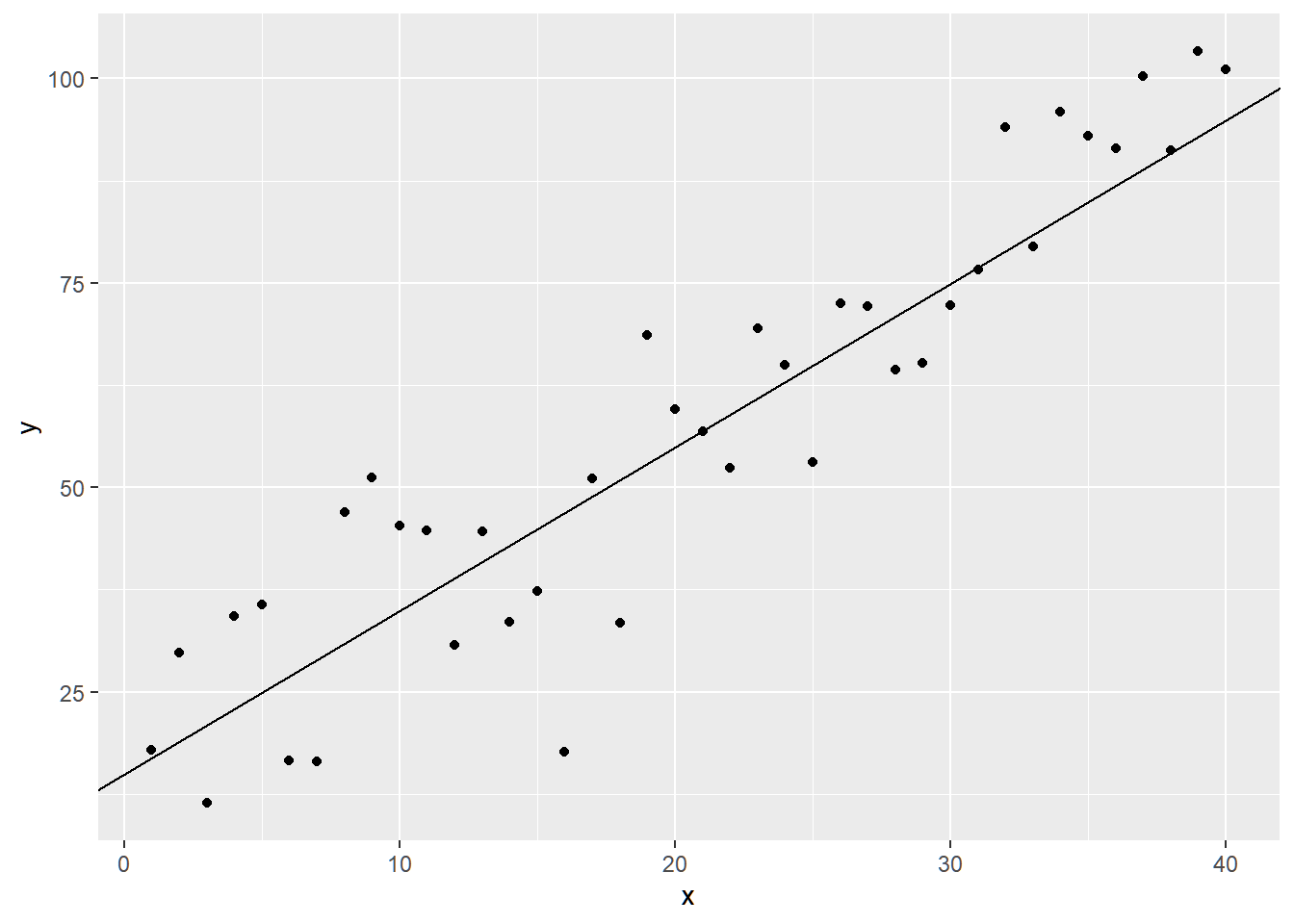
To visualize, let the random variable \(Y_i\) be defined by the equation and random process \[ Y_i=15+2X_i+\varepsilon_i,\quad \quad \varepsilon_i\sim N(0,\sigma=10) \]
x     <- 1:40 # assume that x are predetermined
error <- rnorm(40,0,10) # we can't observe these values naturally in the real world.
y     <- 15 + 2*x + error
We plot the points \(Y_i\) and the theoretical line without the errors \(y=15 + 2x\)
ggplot()+
    geom_point(aes(x=x,y=y)) +        # points (y_i, x_i)
    geom_abline(intercept=15,slope=2) # line of y = 15+2x
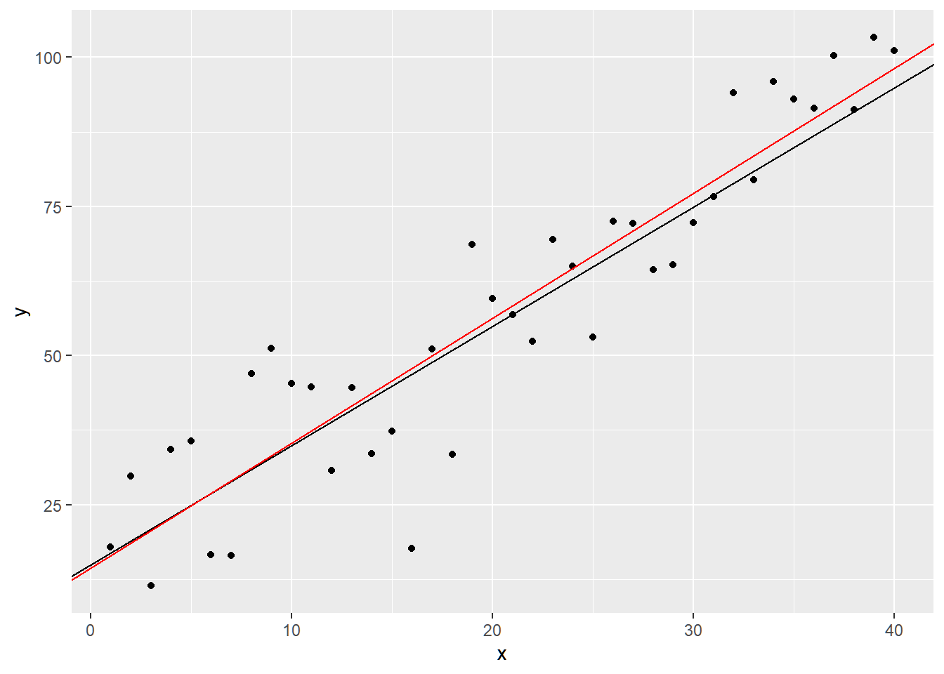
Now, we fit a line that passes through the center of the points using OLS estimation of the regression coefficients.
##
## Call:
## lm(formula = y ~ x)
##
## Coefficients:
## (Intercept)            x
##      14.461        2.095
Now, plotting the fitted line \(\hat{y}=\hat{\beta_0}+\hat{\beta_1}x\)
ggplot() +

    # points (y_i, x_i)
    geom_point(aes(x=x,y=y)) +

    # line of y = 15+2x
    geom_abline(intercept=15,slope=2) +

    # fitted line
    geom_abline(intercept=coef(mod)[1], slope=coef(mod)[2], color = "red")
The error \(\varepsilon_i\) is the (vertical) distance between the black line and the point \(y_i\).
The residual \(e_i\) is the (vertical) distance between the red line and the point \(y_i\). The values will also depend on the line estimation procedure that will be used.
The following table summarizes the dataset used, the errors, and the residuals.
y x error residual 17.92718 1 0.9271800 1.3707302 29.77410 2 10.7740988 11.1226463 11.37954 3 -9.6204598 -9.3669150 34.26851 4 11.2685074 11.4270495 35.71456 5 10.7145588 10.7780982 16.56321 6 -10.4367921 -10.4682554 16.46036 7 -12.5396399 -12.6661059 46.95552 8 15.9555193 15.7340506 51.19369 9 18.1936909 17.8772195 45.26432 10 10.2643215 9.8528474 44.67969 11 7.6796922 7.1732154 30.69876 12 -8.3012425 -8.9027219 44.60956 13 3.6095557 2.9130735 33.52579 14 -9.4742105 -10.2656954 37.33750 15 -7.6624963 -8.5489839 17.63080 16 -29.3691963 -30.3506866 51.04198 17 2.0419765 0.9654836 33.42656 18 -17.5734427 -18.7449384 68.57538 19 15.5753827 14.3088843 59.53468 20 4.5346768 3.1731758 56.79188 21 -0.2081218 -1.6646255 52.34828 22 -6.6517223 -8.2032287 69.42828 23 8.4282821 6.7817729 64.96512 24 1.9651198 0.2236080 53.03037 25 -11.9696337 -13.8061483 72.54908 26 5.5490839 3.6175666 72.18195 27 3.1819465 1.1554266 64.42233 28 -6.5776689 -8.6991915 65.21981 29 -7.7801873 -9.9967126 72.25427 30 -2.7457336 -5.0572616 76.62753 31 -0.3724703 -2.7790010 94.04006 32 15.0400592 12.5385258 79.48937 33 -1.5106341 -4.1071702 95.95420 34 12.9542037 10.2626649 93.01689 35 8.0168946 5.2303531 91.47995 36 4.4799452 1.5984011 100.30822 37 11.3082246 8.3316777 91.23667 38 0.2366726 -2.8348769 103.30805 39 10.3080461 7.1414939 101.14611 40 6.1461089 2.8845539
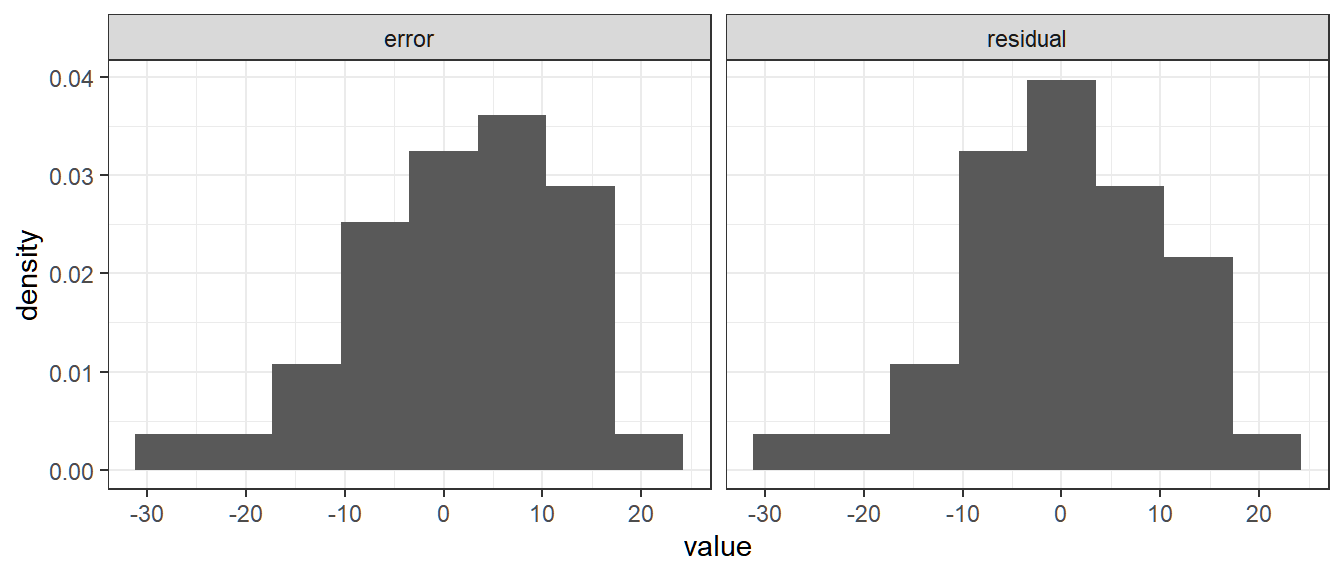
The following relative frequency histograms of the error and the residuals show that they almost follow the same shape.
The closer the fitted line to the theoretical line is, the more likely that the two histograms will look identical
Theorems
The following theorems will be important for later results. Try to prove them all as your practice.
Theorem 4.1 \[ \hat{\boldsymbol{\beta}}=\boldsymbol{\beta}+(\textbf{X}'\textbf{X})^{-1}\textbf{X}'\boldsymbol{\varepsilon} \] That is, the OLS estimator can be thought of as a linear function of the error terms and the model parameters.
Theorem 4.2 The sum of the observed values \(Y_i\) is equal to the sum of the fitted values \(\hat{Y_i}\)
\[
\sum_{i=1}^nY_i=\sum_{i=1}^n\hat{Y_i}
\]
Hint for Proof
Use the first normal equation in OLS
Theorem 4.3 The expected value of the vector of residuals is a null vector. That is, \[ E(\textbf{e})=\textbf{0} \]
Theorem 4.4 The sum of the squared residual is a minimum. That is, \(\textbf{e}'\textbf{e}\) is the minimum value of \(\boldsymbol\varepsilon'\boldsymbol\varepsilon\)
Theorem 4.5 The sum of the residuals in any regression model that with an intercept \(\beta_0\) is always equal to 0. \[ \sum_{i=1}^n e_i = \textbf{1}'\textbf{e} = \textbf{e}'\textbf{1}=0 \]
Hint for Proof
Use the Theorem 4.2
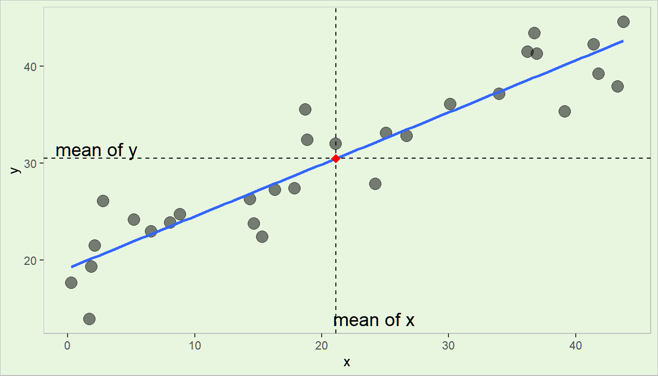
Theorem 4.6 The least squares regression line always passes through the centroid (the point comprising of the means of the dependent and independent variables). That is, if \((\bar{y},\bar{x_1},\bar{x_2},\cdots,\bar{x_k})\) is the centroid of the the dataset, the following equation is true: \[ \bar{y}=\hat{\beta}_0 + \hat{\beta}_1 \bar{x}_1 + \hat{\beta}_2 \bar{x}_2 +\cdots + \hat{\beta}_k \bar{x}_k \]
Visualization
Theorem 4.7 The sum of the residuals weighted by the corresponding value of the regressor variable is always equal to zero. That is,
\[
\sum_{i=1}^nX_{ij}e_{ij}=0 \quad \text{or}
\quad \textbf{X}'\textbf{e}=\textbf{0}
\]
Hint for Proof
Use result from Theorem 4.5, then use the 2nd to (k+1)th normal equations. For every variable \(X_{ij}\), use equation \(j+1\).
Theorem 4.8 The sum of the residuals weighted by the corresponding value of the fitted value is always equal to 0. That is, \[ \sum_{i=1}^n\hat{Y_i}e_i=\textbf{e}'\hat{\textbf{Y}}=0 \]
Hint for Proof
Use previous theorem on sum of residual \(e_j\) and sum of residual \(e_i\) weighted by \(X_{ij}\)
Theorem 4.9
The residual and independent variables are uncorrelated. That is, assuming that \(Xs\) are random again, \[ \rho(X_{ij},e_{ij})=0 \]
Theorem 4.10 The residual and the fitted values are uncorrelated.
\[ \rho(\hat{Y_i},e_i)=0 \]
Remarks:
- One reason why the \(X\)s are required to be uncorrelated (or linearly independent to each other) is to ensure proper conditioning of \(\textbf{X}'\textbf{X}\) and hence, stability of the inverse that will imply stability of the parameter estimates.
- Note that aside from estimating \(\boldsymbol{\beta}\), we also need to estimate \(\sigma^2\) to make inferences regarding the model parameters.
- Before we estimate \(\sigma^2\), we need to discuss first the the sum of squares of the regression analysis.
.
4.2 Analysis of Variance
- Because of the assumption of normality of the error terms, we can now do inferences in regression analysis.
- In particular, one of our interest is in doing an analysis of variance.
- This will help us assess whether we attained our aim in modeling: to explain the variation in \(Y\) in terms of the \(X\)s.
GOAL: In this section, we will show a test for the hypotheses:
\[ Ho: \beta_1=\beta_2,...,\beta_k=0 \quad \text{vs}\quad Ha:\text{at least one }\beta_j\neq0 \text{ for } j=1,2,...,k \]
We want to test if fitting a line on the data is worthwhile. Some preliminaries will be discussed prior to the presentation of the test.
Definition 4.4 In analysis of variance (ANOVA), the total variation displayed by a set of observations, as measured by the sum of squares of deviations from the mean, are separated into components associated with defined sources of variation used as criteria of classification for observations.
Remarks:
An ANOVA decomposes the variation in \(Y\) into those that can be explained by the model and the unexplained portion.
There is variation in \(\textbf{Y}\) as in all statistical data. If all \(Y_i\)s were identically equal, in which case, \(Y_i = \bar{Y}\) for all \(i\), there would be no statistical problems (but not realistic!).
The variation of the \(Y_i\) is conventionally measured in terms of \(Y_i − \bar{Y}\).
Sum of Squares
The ANOVA approach is based on the partitioning variations using sums of squares and degrees of freedom associated with the response variable \(Y\). We start with the observed deviations of \(Y_i\) around the observed mean: \(Y_i-\bar{Y}\).
Definition 4.5 (Total Sum of Squares) The measure of total variation is denoted by \[ SST =\sum_{i=1}^n (Y_i-\bar{Y})^2 \]
- \(SST\) is the total corrected sum of squares
- If all \(Y_i\)s are the same, then \(SST=0\)
- The greater the variation of \(Y_i\)s, the greater \(SST\)
- In ANOVA, we want to find the source of this variation
Now, recall that \(\hat{Y_i}\) is the fitted or values. Other than the variation of the observed \(Y\), we can also measure the variation of the \(\hat{Y_i}\). Note that the mean of the fitted values is also \(\bar{Y}\). We can now explore the deviation \(\hat{Y_i}-\bar{Y}\)
Definition 4.6 (Regression Sum of Squares) The measure of variation of the fitted values due to regression is denoted by \[ SSR = \sum_{i=1}^n (\hat{Y_i}-\bar{Y})^2 \]
- \(SSR\) is the sum of squares due to regression
- This measures the variability of \(Y\) associated with the regression line or due to changes in the independent variables.
- Sometimes referred to as “explained sum of squares”
Finally, recall that the quantity \(Y_i-\hat{Y_i}\) is the residual, or the difference between the observed values and the predicted values when the independent variables are taken into account.
Definition 4.7 (Sum of Squared Deviations) The measure of variation of the \(Y_i\)s that is still present when the predictor variable \(X\) is taken into account is the sum of the squared deviations
\[ SSE=\sum_{i=1}^n(Y_i-\hat{Y_i})^2 \]
- \(SSE\) is the sum of squares due to error
- Mathematically, the formula is the sum of squares of the residuals \(e_i\), not the error. That is why some software outputs show “Sum of Squares from Residuals”.
- It still measures the variability of \(Y\) due to causes other than the set of independent variables.
- Sometimes referred to as ”unexplained sum of squares”
- If the independent variables predict the response variable well, then this quantity is expected to be small.
Theorem 4.11 Under the least squares theory, the sum of squares can be partitioned as \[ \sum_{i=1}^n(Y_i-\bar{Y})^2=\sum_{i=1}^n(\hat{Y_i}-\bar{Y_i})^2+\sum_{i=1}^n(Y_i-\hat{Y_i})^2 \]
Proof
First express \(Y_i-\bar{Y}\) as a sum of two differences by adding and subtracting \(\hat{Y_i}\), then square both sides.
\[\begin{align} (Y_i-\bar{Y})^2 &= [(Y_i-\bar{Y})+(\hat{Y_i}-\hat{Y_i})]^2\\ &= [(Y_i-\hat{Y_i}) + (\hat{Y_i}-\bar{Y})]^2\\ &= (Y_i-\hat{Y_i})^2+(\hat{Y_i}-\bar{Y})^2 + 2(Y_i-\hat{Y_i})(\hat{Y_i}-\bar{Y})\\ &= (Y_i-\hat{Y_i})^2+(\hat{Y_i}-\bar{Y})^2 + 2(Y_i-\hat{Y_i})\hat{Y_i} - 2(Y_i-\hat{Y_i})\bar{Y}\\ &= (Y_i-\hat{Y_i})^2+(\hat{Y_i}-\bar{Y})^2 + 2 e_i \hat{Y_i} - 2 e_i \bar{Y} \end{align}\]
Now getting summation of both sides.
\[\begin{align} \sum_{i=1}^n(Y_i-\bar{Y})^2 &=\sum_{i=1}^n(Y_i-\hat{Y_i})^2 + \sum_{i=1}^n(\hat{Y_i}-\bar{Y})^2 +2\sum_{i=1}^n e_i \hat{Y_i}+2\bar{Y}\sum_{i=1}^n e_i \\ &=\sum_{i=1}^n(Y_i-\hat{Y_i})^2 + \sum_{i=1}^n(\hat{Y_i}-\bar{Y})^2\end{align}\]
Since \(\sum_{i=1}^n\hat{Y}_ie_i=0\) and \(\sum_{i=1}^ne_i=0\) from Theorems 4.8 and 4.5 respectively.
\(\blacksquare\)
Matrix form of the sums of squares
- \(SST=(\textbf{Y}-\bar{Y}\textbf{1})'(\textbf{Y}-\bar{Y}\textbf{1})\)
- \(SSR = (\hat{\textbf{Y}}-\bar{Y}\textbf{1})'(\hat{\textbf{Y}}-\bar{Y}\textbf{1})\)
- \(SSE = (\textbf{Y}-\hat{\textbf{Y}})'(\textbf{Y}-\hat{\textbf{Y}})\)
Exercise 4.1 Show the following (quadratic form of the sum of squares):
- \(SST = \textbf{Y}'(\textbf{I}-\bar{\textbf{J}})\textbf{Y}\)
- \(SSR = \textbf{Y}'(\textbf{H}-\bar{\textbf{J}})\textbf{Y}\)
- \(SSE = \textbf{Y}'(\textbf{I}-\textbf{H})\textbf{Y}\)
Breakdown of Degrees of Freedom
Let \(p=k+1\), the number of coefficients to be estimated (\(\beta_0,\beta_1,...,\beta_k\)) , or the number of columns in the design matrix.
- \(SST=\sum_{i=1}^n(Y_i-\bar{Y})^2\)
- \(n\) observations but \(1\) linear constraint due to the calculation and inclusion of the mean
- \(n-1\) degrees of freedom
- \(SSR=\sum_{i=1}^n(\hat{Y_i}-\bar{Y})^2\)
- \(p\) degrees of freedom in the regression parameters, one is lost due to linear constraint
- \(p-1\) degrees of freedom
- \(SSE=\sum_{i=1}^n(Y_i-\hat{Y_i})^2\)
- \(n\) independent observations but \(p\) linear constraints arising from the estimation of \(\beta_0,\beta_1,...,\beta_k\)
- \(n-p\) degrees of freedom
Just accept the degrees of freedom for now.
In classical linear regression, the degrees of freedom associated with a quadratic form involving \(\textbf{Y}\) is equal to the rank of the matrix involved in the quadratic form, which will be discussed further in Stat 147.
Mean Squares
Definition 4.8 (Mean Squares) The mean squares in regression are the sum of squares divided by their corresponding degrees of freedom. \[ MST = \frac{SST}{n-1}\quad MSR = \frac{SSR}{p-1} \quad MSE = \frac{SSE}{n-p} \]
Theorem 4.12 (Expectation of MSE and MSR) \[ E(MSE)=\sigma^2,\quad E(MSR)=\sigma^2+\frac{1}{p-1}(\textbf{X}\boldsymbol\beta)'(\textbf{I}-\bar{\textbf{J}})\textbf{X}\boldsymbol{\beta} \]
Exercise 4.2 Prove Theorem 4.12
Sampling Distribution of the Sum of Squares while Assuming Same Means of \(Y_i|\textbf{x}\)
Before we proceed with constructing the hypothesis test, we need to define the sampling distribution of the statistics that we will use.
Theorem 4.13 (Cochran's Theorem) If all \(n\) observations \(Y_i\) come from the same normal distribution with same mean \(\mu\) and variance \(\sigma^2\) and \(SST\) is decomposed into k sums of squares \(SS_j\) , each with \(\text{df}_j\) , then the \(\frac{SS_j}{\sigma^2}\) terms are independent \(\chi^2\) random variables with \(\text{df}_j\) if the sum of the \(\text{df}_j\)s = \(\text{df}\) of SST= \(n-1\) .
If all observations comes from the same normal distribution with SAME PARAMETERS regardless of \(i\), that is \(Y_i\sim N(\beta_0,\sigma^2)\), then
\[ \frac{SST}{\sigma^2} \sim \chi^2_{(n-1)} \quad \frac{SSR}{\sigma^2} \sim \chi^2_{(p-1)} \quad \frac{SSE}{\sigma^2} \sim \chi^2_{(n-p)} \]
Exercise 4.3 Find the expected value of the \(MSR\) and \(MSE\) while assuming \(Y_i\sim N(\beta_0,\sigma^2)\).
Use properties of a \(\chi^2\) random variable, NOT Theorem 4.12.
This exercise shows that if \(\beta_1=\beta_2=\cdots=\beta_k=0\), then \(MSE\) and \(MSR\) will approach some relationship. Interpret your findings.
ANOVA Table and F Test for Regression Relation
| Source of Variation | df | Sum of Squares | Mean Square | F-stat | p-value |
|---|---|---|---|---|---|
| Regression | \(p-1\) | \(SSR\) | \(MSR\) | \(F_c=\frac{MSR}{MSE}\) | \(P(F>F_c)\) |
| Error | \(n-p\) | \(SSE\) | \(MSE\) | ||
| Total | \(n-1\) | \(SST\) |
The ANOVA table is a classical result that is always presented in regression analysis.
It is a table of results that details the information we can extract from doing the F-test for Regression Relation (oftentimes simply referred to as the F-test for ANOVA).
The said test has the following competing hypotheses:
\[ Ho: \beta_1=\beta_2,...,\beta_k=0 \quad vs\quad Ha:\text{at least one }\beta_j\neq0 \text{ for } j=1,2,...,k \]
It basically tests whether it is still worthwhile to do regression on the data.
Definition 4.9 (F-test for Regression Relation)
For testing \(Ho: \beta_1=\beta_2,...,\beta_k=0\) vs \(Ha:\text{at least one }\beta_j\neq0 \text{ for } j=1,2,...,k\), the test statistic is
\[ F_c=\frac{MSR}{MSE}=\frac{SSR/(p-1)}{SSE/(n-p)}\sim F_{(p-1),(n-p)},\quad \text{under } Ho \]
The critical region of the test is \(F_c>F^\alpha_{(p-1),(n-p)}\)
More details about this test in [Testing all slope parameters equal to 0]
Example in R
We use the data by F.J. Anscombe again which contains U.S. State Public-School Expenditures in 1970.
| education | income | young | urban | |
|---|---|---|---|---|
| ME | 189 | 2824 | 350.7 | 508 |
| NH | 169 | 3259 | 345.9 | 564 |
| VT | 230 | 3072 | 348.5 | 322 |
| MA | 168 | 3835 | 335.3 | 846 |
| RI | 180 | 3549 | 327.1 | 871 |
| CT | 193 | 4256 | 341.0 | 774 |
| NY | 261 | 4151 | 326.2 | 856 |
| NJ | 214 | 3954 | 333.5 | 889 |
| PA | 201 | 3419 | 326.2 | 715 |
| OH | 172 | 3509 | 354.5 | 753 |
| IN | 194 | 3412 | 359.3 | 649 |
| IL | 189 | 3981 | 348.9 | 830 |
| MI | 233 | 3675 | 369.2 | 738 |
| WI | 209 | 3363 | 360.7 | 659 |
| MN | 262 | 3341 | 365.4 | 664 |
| IO | 234 | 3265 | 343.8 | 572 |
| MO | 177 | 3257 | 336.1 | 701 |
| ND | 177 | 2730 | 369.1 | 443 |
| SD | 187 | 2876 | 368.7 | 446 |
| NE | 148 | 3239 | 349.9 | 615 |
| KA | 196 | 3303 | 339.9 | 661 |
| DE | 248 | 3795 | 375.9 | 722 |
| MD | 247 | 3742 | 364.1 | 766 |
| DC | 246 | 4425 | 352.1 | 1000 |
| VA | 180 | 3068 | 353.0 | 631 |
| WV | 149 | 2470 | 328.8 | 390 |
| NC | 155 | 2664 | 354.1 | 450 |
| SC | 149 | 2380 | 376.7 | 476 |
| GA | 156 | 2781 | 370.6 | 603 |
| FL | 191 | 3191 | 336.0 | 805 |
| KY | 140 | 2645 | 349.3 | 523 |
| TN | 137 | 2579 | 342.8 | 588 |
| AL | 112 | 2337 | 362.2 | 584 |
| MS | 130 | 2081 | 385.2 | 445 |
| AR | 134 | 2322 | 351.9 | 500 |
| LA | 162 | 2634 | 389.6 | 661 |
| OK | 135 | 2880 | 329.8 | 680 |
| TX | 155 | 3029 | 369.4 | 797 |
| MT | 238 | 2942 | 368.9 | 534 |
| ID | 170 | 2668 | 367.7 | 541 |
| WY | 238 | 3190 | 365.6 | 605 |
| CO | 192 | 3340 | 358.1 | 785 |
| NM | 227 | 2651 | 421.5 | 698 |
| AZ | 207 | 3027 | 387.5 | 796 |
| UT | 201 | 2790 | 412.4 | 804 |
| NV | 225 | 3957 | 385.1 | 809 |
| WA | 215 | 3688 | 341.3 | 726 |
| OR | 233 | 3317 | 332.7 | 671 |
| CA | 273 | 3968 | 348.4 | 909 |
| AK | 372 | 4146 | 439.7 | 484 |
| HI | 212 | 3513 | 382.9 | 831 |
Our dependent variable is the Per-capita income in dollars
##
## Call:
## lm(formula = income ~ education + young + urban, data = Anscombe)
##
## Residuals:
##     Min      1Q  Median      3Q     Max
## -438.54 -145.21  -41.65  119.20  739.69
##
## Coefficients:
##              Estimate Std. Error t value Pr(>|t|)
## (Intercept) 3011.4633   609.4769   4.941 1.03e-05 ***
## education      7.6313     0.8798   8.674 2.56e-11 ***
## young         -6.8544     1.6617  -4.125  0.00015 ***
## urban          1.7692     0.2591   6.828 1.49e-08 ***
## ---
## Signif. codes:  0 '***' 0.001 '**' 0.01 '*' 0.05 '.' 0.1 ' ' 1
##
## Residual standard error: 259.7 on 47 degrees of freedom
## Multiple R-squared:  0.7979, Adjusted R-squared:  0.785
## F-statistic: 61.86 on 3 and 47 DF,  p-value: 2.384e-16
The F-statistic and the p-value are already shown using the summary() function.
At this point, the ANOVA table is not necessary anymore since result of the F-test is already presented.
For the sake of this example, how do we output the ANOVA table?
## Analysis of Variance Table
##
## Response: income
##           Df  Sum Sq Mean Sq F value    Pr(>F)
## education  1 6988589 6988589 103.658 1.788e-13 ***
## young      1 2381325 2381325  35.321 3.281e-07 ***
## urban      1 3142811 3142811  46.616 1.493e-08 ***
## Residuals 47 3168730   67420
## ---
## Signif. codes:  0 '***' 0.001 '**' 0.01 '*' 0.05 '.' 0.1 ' ' 1
Unfortunately, the output of anova() in R does not directly provide the SST, SSR, and SSE, and the F test of the full model. That is, only Sequential F-tests are presented. See more about this in Testing a slope parameter equal to 0 sequentially
In this example, we can just try to calculate the important figures manually.
Y    <- Anscombe$income
Ybar <- mean(Anscombe$income)
Yhat <- fitted(mod_anscombe)

SST  <- sum((  Y  - Ybar)^2)  # Total Sum of Squares
SSR  <- sum((Yhat - Ybar)^2)  # Regression Sum of Squares
SSE  <- sum((Yhat -   Y )^2)  # Error Sum of Squares

n    <- nrow(Anscombe)
p    <- length(coefficients(mod_anscombe))

MSR  <- SSR/(p-1)
MSE  <- SSE/(n-p)

F_c  <- MSR/MSE
Pr_F <- pf(F_c,p-1,n-p, lower.tail = F)| Source | df | Sum_of_Squares | Mean_Square | F_value | Pr_F |
|---|---|---|---|---|---|
| Regression | 3 | 12512724.9115 | 4170908.3038 | 61.8648 | <0.0001 |
| Error | 47 | 3168729.6767 | 67419.7804 | ||
| Total | 50 | 15681454.5882 |
At 0.05 level of significance, there is sufficient evidence to conclude that there is at least one \(\beta_j\neq0\).
Exercise 4.4 Assuming normality of errors, show that the statistic \(F_c\) follows the \(F\) distribution with degrees of freedom \(\nu_1=p-1\) and \(\nu_2=n-p\) under the null hypothesis.
Hints
- What is the null hypothesis?
- If the null hypothesis is true, can we use Cochran’s Theorem?
- Recall results in sampling from the normal distribution
4.3 Estimation of the Error Variance
Now that we already finished the discussion on ANOVA, we now have a means on estimating the error term variance \(\sigma^2\) and the variance of the model parameter OLS estimator.
Theorem 4.14 The MSE is an unbiased estimator of \(\sigma^2\). \[ E\left(\frac{1}{n-p}\sum_{i=1}^n e_i^2\right)=\sigma^2 \]
Remarks:
Recall that \(Var(\hat{\boldsymbol\beta})=\sigma^2(\textbf{X}'\textbf{X})^{−1}\) from Theorem 3.3.
With the theorem above, a possible estimator of \(Var(\hat{\boldsymbol\beta})\) is given by \[\widehat{Var(\hat{\boldsymbol{\beta}})} = \widehat{\sigma^2}(\textbf{X}'\textbf{X})^{−1}=MSE (\textbf{X}'\textbf{X})^{−1} \]
This also implies that an estimator for the standard deviation of \(\hat{\beta_j}\) is the square root of the \((j+1)^{th}\) diagonal element of \(\widehat{Var}({\hat{\boldsymbol{\beta}}})\). In matrix form: \[ \widehat{s.e\left(\hat{\beta}_j\right)}=\sqrt{\underline{e}_{j+1}'\widehat{Var}({\hat{\boldsymbol{\beta}}})\underline{e}_{j+1}}=\sqrt{MSE\underline{e}_{j+1}'(\textbf{X}'\textbf{X})^{−1}\underline{e}_{j+1}} \] where \(\underline{e}_k\) is a vector of \(0\)s with \(1\) on the \(k^{th}\) element.
More properties regarding MSE as an estimator of \(\sigma^2\) will be discussed later in Section 4.5.
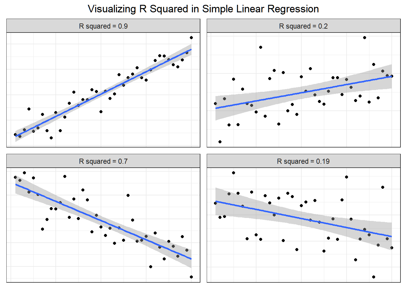
4.4 Coefficient of Multiple Determination
Definition 4.10 (Coefficient of Multiple Determination) The coefficient of multiple determination of Y associated with the use of the set of independent variables \((X_1, X_2, . . . , X_k )\) denoted by \(R^2\) or \(R^2_{Y.1,2,...,k}\) is defined as \[ R^2=R^2_{Y.1,2,...,k}=\frac{SSR(X_1,X_2,...,X_k)}{SST}=1-\frac{SSE(X_1,X_2,...,X_k)}{SST} \]
Remarks:
The coefficient of multiple determination measures the percentage of variation in Y than can be explained by the X’s through the model.
For \(R^2\), the larger the better. However, high value of \(R^2\) does not imply usefulness of the model.
\(R^2\) increases as more variables are included in the model (cross-classified data)
\(0 \leq R^2 \leq 1\)
\(R^2 = r^2\) when \(k = 1\), where \(r\) is the Pearson’s r
If the intercept is dropped from the model, \(R^2 = SSR/SST\) is an incorrect measure of coefficient of determination.
Exercise 4.5
Read: What is overfitting?
In statistical modelling, there is this problem called “overfitting”. This occurs if the model becomes more deterministic that it may not describe the statistical relationship of the dependent and independent variables.
Common indication for this is too high \(R^2\) (close to 1).
This further implies that the model is good for the collected data, but may not perform well for new data. A good statistical model must have enough elbow room for possible errors in data.
In the following exercise, we show that overfitting exists for a specific case based on the number of observed values in the collected dataset.
Suppose that the observed values for your dependent variable are not constant and the observed values of the independent variables are linearly independent.
Show that if the number of observations and number of parameters to be estimated are equal to each other (\(n=p\)), then \(R^2=1\)
There are also other measures related to the \(R^2\).
Definition 4.11 (Cofficient of Alienation) The coefficient of alienation (non-determination) is the proportion of variation in \(Y\) that is not explained by the set of independent variables
Recall that as more variables are included in the model, it is expected that the \(R^2\) increases. We do not want this, since we want to penalize adding variables that do not explain the dependent variable well. The following definition is a more conservative measure of coefficient of determination.
Definition 4.12 (Adjusted Coefficient of Determination) The adjusted coefficient of determination denoted by \(R_a^2\) is defined as
\[ R^2_a=1-\frac{MSE}{MST}=1-\frac{SSE/(n-p)}{SST/(n-1)} \]
Example in R
In R, both the Multiple R-squared and Adjusted R-squared are shown using the summary() function. In this example, note that mod_anscombe is an lm object from the ANOVA example.
##
## Call:
## lm(formula = income ~ education + young + urban, data = Anscombe)
##
## Residuals:
##     Min      1Q  Median      3Q     Max
## -438.54 -145.21  -41.65  119.20  739.69
##
## Coefficients:
##              Estimate Std. Error t value Pr(>|t|)
## (Intercept) 3011.4633   609.4769   4.941 1.03e-05 ***
## education      7.6313     0.8798   8.674 2.56e-11 ***
## young         -6.8544     1.6617  -4.125  0.00015 ***
## urban          1.7692     0.2591   6.828 1.49e-08 ***
## ---
## Signif. codes:  0 '***' 0.001 '**' 0.01 '*' 0.05 '.' 0.1 ' ' 1
##
## Residual standard error: 259.7 on 47 degrees of freedom
## Multiple R-squared:  0.7979, Adjusted R-squared:  0.785
## F-statistic: 61.86 on 3 and 47 DF,  p-value: 2.384e-16
Using the Adjusted \(R^2\), 78.5% of the variation in income can be explained by the model.
4.5 Properties of the Estimators of the Regression Parameters
In the following section, we will show that the OLS estimator \(\hat{\boldsymbol{\beta}}\) is also the BLUE, MLE, and UMVUE of \(\boldsymbol{\beta}\). Estimators for the variance \(\sigma^2\) are presented as well.
Note that this section does not just introduce other estimators, but also demonstrates the characterization and properties of the estimators.
Best Linear Unbiased Estimator of \(\boldsymbol{\beta}\)
Theorem 4.15 (Gauss-Markov Theorem)
Under the classical conditions of the multiple linear regression model (i.e., \(E(\boldsymbol{\varepsilon}) = \textbf{0}\), \(Var(\boldsymbol{\varepsilon}) = \sigma^2\textbf{I}\), not necessarily normal), the least squares estimator \(\hat{\boldsymbol\beta}\) is the best linear unbiased estimator (BLUE) of \(\boldsymbol{\beta}\). This means that among all linear unbiased estimators of \(\beta_j\), \(\hat{\beta_j}\) has the smallest variance, \(j = 0, 1, 2, ..., k\).
Hint for Proof
“OLS will have the smallest possible variance among other linear unbiased estimators.”
Consider any linear estimator of the coefficient vector \(\boldsymbol{\beta}\), say \(\overset{\sim}{\boldsymbol\beta}=\textbf{CY}\) .
Show that if \(E(\overset{\sim}{\boldsymbol\beta})=\boldsymbol{\beta}\) (unbiased), then \(Var(\overset{\sim}{\boldsymbol\beta})-Var(\hat{\boldsymbol{\beta}})\) is a positive semi-definite matrix.
Remarks:
- The Gauss-Markov Theorem states that even though the error terms are not normally distributed, the OLS estimator is still a viable estimator for linear regression.
- The OLS estimator will give the smallest possible variance among all linear unbiased estimators of \(\boldsymbol\beta\)
- Any linear combination \(\boldsymbol{\lambda}'\boldsymbol\beta\) of the elements of \(\boldsymbol\beta\), the BLUE is \(\boldsymbol{\lambda}'\hat{\boldsymbol\beta}\)
Maximum Likelihood Estimator of \(\boldsymbol{\beta}\) and \(\sigma^2\)
Theorem 4.16 (MLE of the Regression Coefficients and the Variance)
With assumptions of normality of the error terms, the maximum likelihood estimators (MLE) for \(\boldsymbol{\beta}\) and \(\sigma^2\) are \[
\hat{\boldsymbol{\beta}}=(\textbf{X}'\textbf{X})^{-1}(\textbf{X}'\textbf{Y})
\quad \quad \quad
\widehat{\sigma^2}=\frac{1}{n}\textbf{e}'\textbf{e}=\frac{SSE}{n}=\left(\frac{n-p}{n} \right)MSE
\]
Hint for Proof
Recall: \(Y_i \sim Normal(\textbf{x}_i'\boldsymbol{\beta},\sigma^2)\)
Note: the likelihood function is just the joint pdf, but a function of the parameters, given the values of the random variables.
Since \(Y_i\)s are independent, the joint pdf of \(Y_i\)s is the product
\[ \prod_{i=1}^n f(Y_i)=\prod_{i=1}^n \frac{1}{\sqrt{2\sigma^2}}\exp\left\{-\frac{(Y_i-\textbf{x}'_i\boldsymbol{\beta})^2}{2\sigma^2}\right\} \]
Hence, you can show that the likelihood function is given by \[ L(\boldsymbol{\beta},\sigma^2|\textbf{Y},\textbf{X})=(2\pi \sigma^2)^{-\frac{n}{2}}\exp\left\{ -\frac{1}{2\sigma^2}(\textbf{Y}-\textbf{X}\boldsymbol{\beta})'(\textbf{Y}-\textbf{X}\boldsymbol{\beta})\right\} \] Obtain the log-likelihood function (for easier maximization).
The maximum likelihood estimator for \(\boldsymbol{\beta}\) and \(\sigma^2\) are the solutions to the following equations: \[ \frac{\partial\ln(L)}{\partial \boldsymbol{\beta}}=\textbf{0} \quad \frac{\partial\ln(L)}{\partial \sigma^2}=0 \quad \]
Remarks:
- We interpret these as the “most likely values” of \(\boldsymbol{\beta}\) and \(\sigma^2\) given our sample (hence the name maximum likelihood).
- The form implies that the MLE estimator for \(\boldsymbol\beta\) is also the OLS \(\hat{\boldsymbol\beta}\) that we showed in Theorem 3.1.
- Recall that MSE is unbiased for \(\sigma^2\) from Theorem 4.12 and obviously, MSE is not the MLE for \(\sigma^2\). Therefore, the MLE estimator of \(\sigma^2\) is not unbiased with respect to \(\sigma^2\).
- The MLE is rarely used in practice; MSE is the conventional estimator for \(\sigma^2\).
UMVUE of \(\boldsymbol{\beta}\) and \(\sigma^2\)
Theorem 4.17 (UMVUE of the Regression Coefficients and Variance)
Under the assumption of normal error terms, \((\hat{\beta},MSE)\) is the uniformly minimum variance unbiased estimator (UMVUE) of \((\boldsymbol{\beta} ,\sigma^2)\)
Hint for Proof
We have established that \(\hat{\boldsymbol{\beta}}\) and \(MSE\) are unbiased estimators for \(\boldsymbol{\beta}\) and \(\sigma^2\) respectively.
Thus, we can just use the Lehmann-Scheffé Theorem to determine a joint complete sufficient statistic for \((\boldsymbol{\beta},\sigma^2)\).
If the unbiased estimator \((\hat{\boldsymbol{\beta}}, MSE)\) is a function of the joint CSS, then that estimator is UMVUE for \((\boldsymbol{\beta},\sigma^2)\)
- This implies that among all other unbiased estimator of \((\boldsymbol\beta, \sigma^2)\), \((\hat{\boldsymbol\beta}, MSE)\) will give the smallest variability (and hence, the ”most precise” or “reliable”).
- The OLS estimator is also the UMVUE for \(\boldsymbol{\beta}\).
| Parameter | OLS | BLUE | MLE | UMVUE |
|---|---|---|---|---|
| \(\boldsymbol\beta\) | \(\hat{\boldsymbol\beta}\) | \(\hat{\boldsymbol\beta}\) | \(\hat{\boldsymbol\beta}\) | \(\hat{\boldsymbol\beta}\) |
| \(\sigma^2\) | - | - | \(\widehat{\sigma^2}=\left(\frac{n-p}{n}\right)MSE\) | \(MSE\) |
4.6 Standardized Coefficients
Note that regression coefficients \(\beta_i\)s are dependent on the unit of measurements of the independent variables. It is difficult to compare regression coefficients because of the differences in the units involved.
Standardized coefficients have been proposed to facilitate comparisons between regression coefficients.
Definition 4.13 (Standardized Coefficients) Standardized \(\beta\) coefficients show how strong and which way variables relate when they’re measured in different units or scales. Standardizing them puts all variables on the same scale, making comparisons easier.
Given the model: \[ Y_i=\beta_0+\beta_1X_1+\cdots +\beta_kX_k + \varepsilon_i \] Standardize each observation by subtracting the mean and dividing by the standard deviation. \[ \frac{Y_i-\mu_Y}{\sigma_Y}=\frac{\beta_1\sigma_1}{\sigma_Y}\frac{(X_1-\mu_1)}{\sigma_1}+\cdots +\frac{\beta_k\sigma_k}{\sigma_Y}\frac{(X_1-\mu_k)}{\sigma_k} + \frac{\varepsilon_i}{\sigma_Y} \]
The new regression model \[ \textbf{Y}^*=\textbf{X}^*\boldsymbol{\beta}^*+\boldsymbol{\varepsilon}^*,\quad \text{where } E(\varepsilon^*_i)=0 \text{ and } V(\varepsilon^*_i)=1 \] where \(\textbf{X}^*\) is a matrix of centered and scaled independent variables.
Theorem 4.18 If \(\textbf{X}^*\) is a matrix of centered and scaled independent variables, and \(\textbf{Y}^*\) is a vector of centered and scaled dependent variable, then
\[ \frac{1}{n-1}{\textbf{X}^*}^T \textbf{X}^*=\textbf{R}_{xx} \quad \quad \frac{1}{n-1}{\textbf{X}^*}^T \textbf{Y}^*=\textbf{R}_{xy} \]
where \(\textbf{R}_{xx}\) is the correlation matrix of independent variables and \(\textbf{R}_{xy}\) is the correlation vector of the dependent variable with each of the independent variables.
Definition 4.14 A scale invariant least squares estimate of the regression coefficients is given by \[\begin{align} \hat{\boldsymbol{\beta}}^* &= (\textbf{X}^{*T}\textbf{X}^*)^{-1}\textbf{X}^{*T}\textbf{Y}^*\\ &= [(n-1)\textbf{R}_{xx}]^{-1}[(n-1)\textbf{R}_{xy}] \end{align}\]
New interpretation: A 1 standard deviation change in \(X_j\) results to a \(\hat{\beta}_j^*\) standard deviation change in \(Y\) \[ \hat{\beta}_j^*=\hat{\beta}_j\frac{s_j}{s_y} \quad \rightarrow \quad \hat{\beta}_j^*s_y=\hat{\beta}_js_j \]
Definition 4.15 (Elasticity) Effect of a percentage change of an independent variable on the dependent variable. \[ E_i=\hat{\beta}_j\frac{\bar{x}_j}{\bar{y}} \]
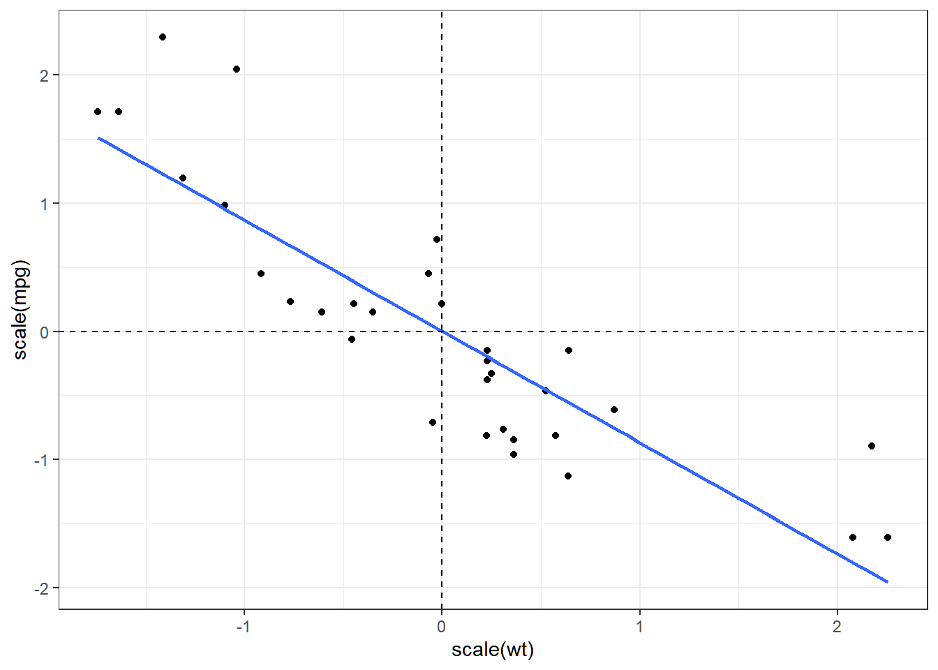
Illustration in R
The scale() function scales and center matrix-like objects, such as vectors, using the following formula.
\[ \frac{X-\bar{X}}{s_x} \]
The following is the visualization of standardized values in simple linear regression. Notice that the centroid of the scaled x and y variables is (0,0).
We can directly apply this function inside the lm() function to standardize the variables before regression.
##
## Call:
## lm(formula = scale(mpg) ~ scale(wt) + scale(cyl), data = mtcars)
##
## Residuals:
##      Min       1Q   Median       3Q      Max
## -0.71169 -0.25737 -0.07771  0.26120  1.01218
##
## Coefficients:
##               Estimate Std. Error t value Pr(>|t|)
## (Intercept)  4.898e-17  7.531e-02   0.000 1.000000
## scale(wt)   -5.180e-01  1.229e-01  -4.216 0.000222 ***
## scale(cyl)  -4.468e-01  1.229e-01  -3.636 0.001064 **
## ---
## Signif. codes:  0 '***' 0.001 '**' 0.01 '*' 0.05 '.' 0.1 ' ' 1
##
## Residual standard error: 0.426 on 29 degrees of freedom
## Multiple R-squared:  0.8302, Adjusted R-squared:  0.8185
## F-statistic: 70.91 on 2 and 29 DF,  p-value: 6.809e-12
Exercise 4.7 In this exercise, we visualize Theorem 4.18 using actual data. Let’s try mtcars, where the dependent variable ismpg, and the independent variables are the rest. Follow these steps in R.
Split the dataframe into vector of dependent variables \(\textbf{Y}\) and matrix of independent variables \(\textbf{X}\).
Y <- as.matrix(mtcars[,1])X <- as.matrix(mtcars[,2:11])
Scale and center all \(\textbf{Y}\) and \(\textbf{X}\) to \(\textbf{Y}^*\) and \(\textbf{X}^*\) respectively. The
scalefunction may help in transforming a matrix per column.Perform the matrix operations \(\frac{1}{n-1}{\textbf{X}^*}^T\textbf{X}^*\) and \(\frac{1}{n-1}{\textbf{X}^*}^T\textbf{Y}^*\)
Obtain correlations \(\textbf{R}_{xx}\) and \(\textbf{R}_{xy}\). You may use the functions
cor(X)andcor(X,Y)respectively.
What can you say about the results of 3 and 4?