3 City-level pollen phenology

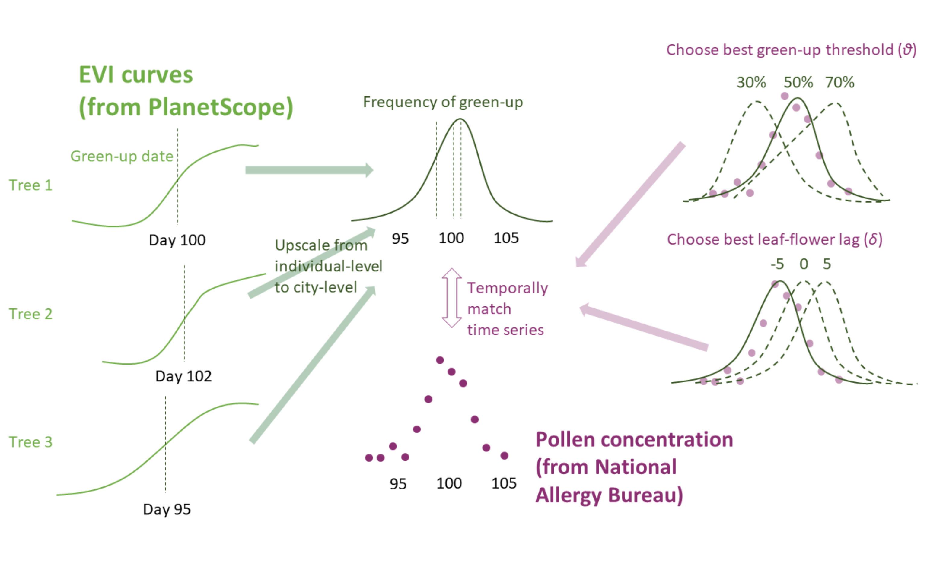
Approach for detecting pollen phenology from remotely-sensed leafing phenology. Enhanced vegetation index (EVI) time series of individual trees are used to determine green-up/down days at various green-up/down thresholds. The green-up/down days were then summarized to the site level as green-up/down frequencies. The green-up/down frequencies were compared with time series of pollen count (squareroot-transformed). For each taxa and across all sites, the green-up/down threshold that lead to the best match in the shapes of leafing and pollen phenology curves was chosen. For each site specifically, the best lag between leafing and pollen phenology curves were chosen.

Figure 3.1: Approach for detecting pollen phenology from remotely-sensed leafing phenology. Enhanced vegetation index (EVI) time series of individual trees are used to determine green-up/down days at various green-up/down thresholds. The green-up/down days were then summarized to the site level as green-up/down frequencies. The green-up/down frequencies were compared with time series of pollen count (squareroot-transformed). For each taxa and across all sites, the green-up/down threshold that lead to the best match in the shapes of leafing and pollen phenology curves was chosen. For each site specifically, the best lag between leafing and pollen phenology curves were chosen.

3.1 NAB data

NAB data were used to calibrate and validate city-level pollen phenology.

Read in data using tidynab package.

source("code/data_nab_read.R")

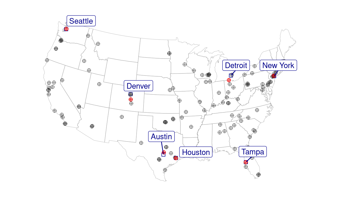
Focus on seven major cities in CONUS with pollen count data and street tree inventory.

Exceptions: Denver pollen data are from Colorado Springs; Austin pollen data are from Georgetown; Detroit pollen data are from Sylvania.

v_site <- c("NY", "AT", "ST", "HT", "TP", "DT", "DV")
v_site_name <- c("New York", "Austin", "Seattle", "Houston", "Tampa", "Detroit", "Denver")
v_site_tune <- c("NY", "AT", "ST", "HT", "TP", "DT", "DV")

Retrieve climatologies (long-term climate) of these cities from TerraClim.

source("code/data_terraclim.R")
df_terraclim

## # A tibble: 7 × 3
##   site    mat   tap
##   <chr> <dbl> <dbl>
## 1 AT    19.4   842.
## 2 DV     9.25  424 
## 3 ST    10.9  1011 
## 4 HT    21.3  1249.
## 5 NY    12.3  1198.
## 6 DT    10.2   869.
## 7 TP    22.6  1298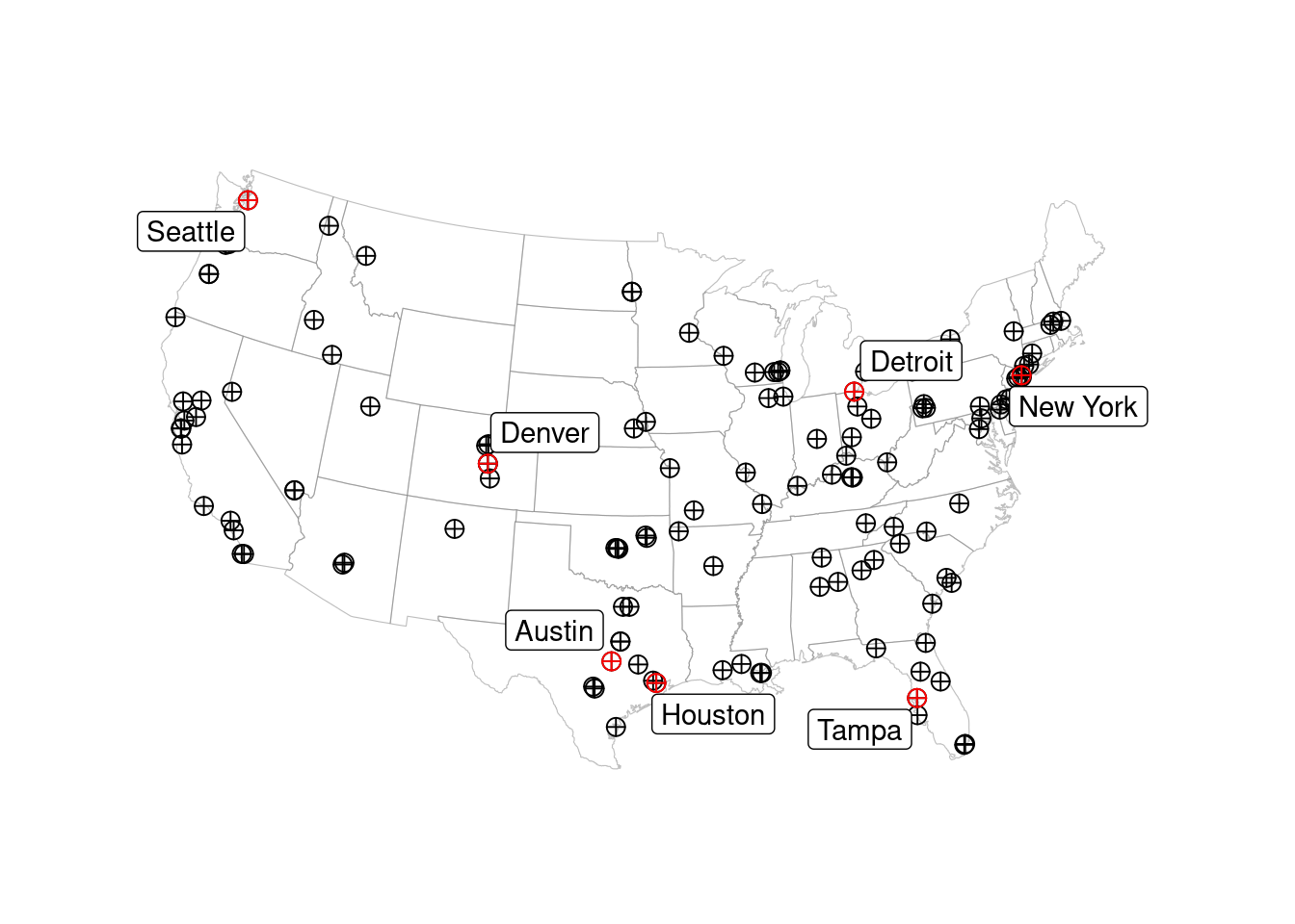

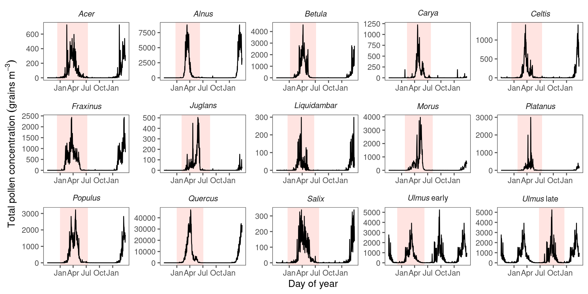
source("code/data_nab_meta.R")
p_pollen_map

source("code/data_nab_avail.R")
p_nab_avail

View pollen phenology in study sites.

source("code/data_nab_pheno.R")
p_nab_calen

Estimate genus-specific pollen seasons by fitting Gaussian kernels.

source("code/data_nab_window.R")
p_flower_window

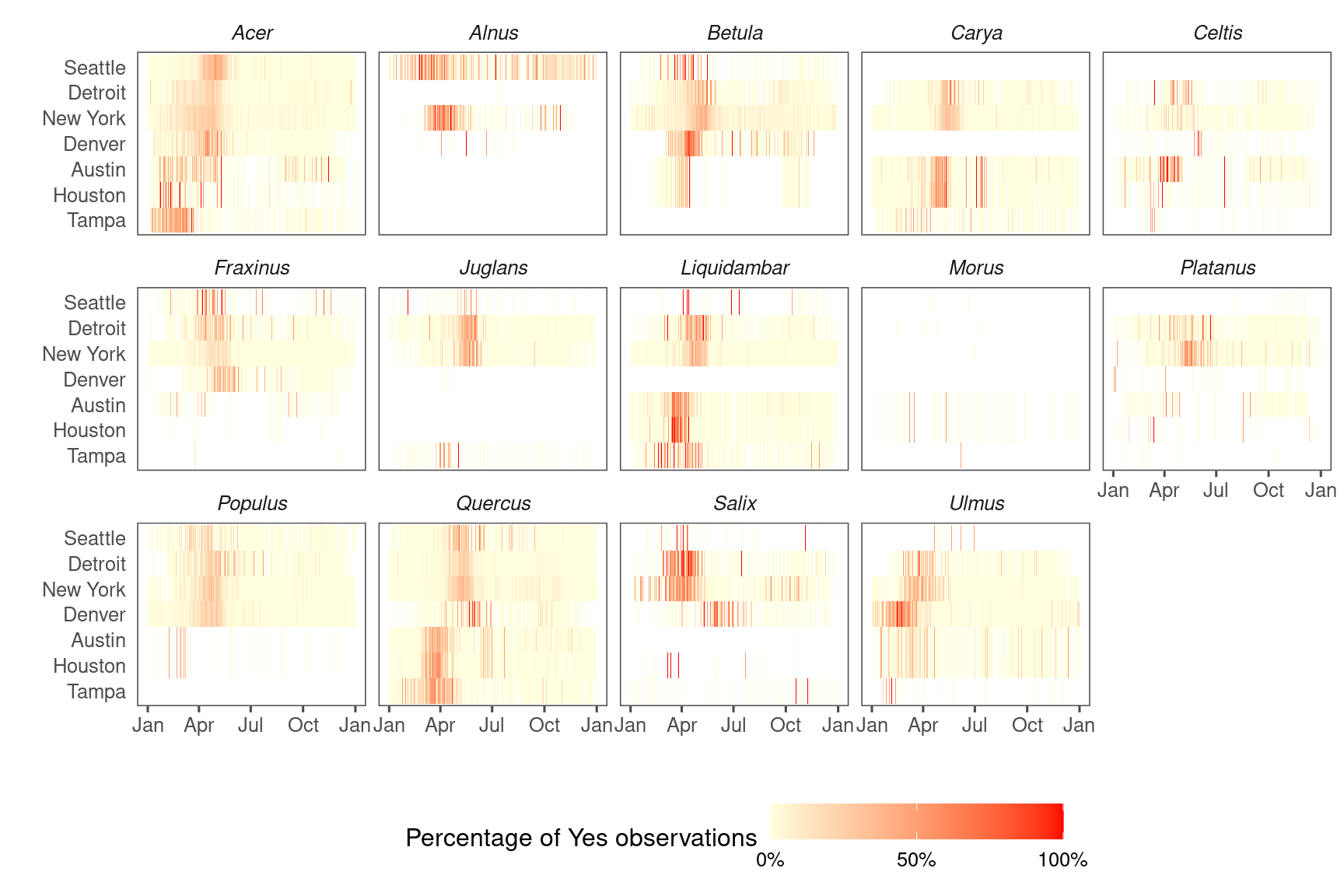
3.2 NPN data

NPN data were used in addition to NAB data to validate city-level pollen phenology.

Download all NPN data for taxa studied.

source("code/data_npn_down.R")

Visualize NPN data and visualize.

source("code/data_npn_pheno.R")
p_npn_calen

3.3 Street tree inventory data

Street tree inventory data from seven cities were compiled to locate pixels of interest for PlanetScope data retrieval.

Read in data previously processed with batchplanet package.

source("code/data_occ_tree_read.R")

Find family names from genus names. This step needs supervision when run for the first time.

source("code/data_occ_tree_taxa.R")

Map relative position of tree inventory and nab station.

source("code/data_occ_map.R")
p_nab_plant_map

Calculate distance from plants to NAB stations in the unit of km.

source("code/data_occ_dist.R")
df_distance

## # A tibble: 7 × 7
##   site  midlon midlat sitelon sitelat sitename distance
##   <chr>  <dbl>  <dbl>   <dbl>   <dbl> <fct>       <dbl>
## 1 AT     -97.7   30.3   -97.7    30.6 Austin      40.9 
## 2 DT     -83.1   42.4   -83.7    41.7 Detroit     90.7 
## 3 DV    -105.    39.7  -105.     38.9 Denver      96.5 
## 4 HT     -95.4   29.7   -95.4    29.7 Houston      4.28
## 5 NY     -73.9   40.7   -74.0    40.8 New York    11.1 
## 6 ST    -122.    47.6  -122.     47.7 Seattle      7.07
## 7 TP     -82.4   28.1   -82.4    28.1 Tampa        3.65

Prepare street map as basemap. Street shapefiles for major cities manually downloaded from https://dataverse.harvard.edu/dataset.xhtml?persistentId=doi:10.7910/DVN/CUWWYJ. Boeing, Geoff, 2017, “U.S. Street Network Shapefiles, Node/Edge Lists, and GraphML Files”, https://doi.org/10.7910/DVN/CUWWYJ, Harvard Dataverse, V2

source("code/data_occ_road_read.R")

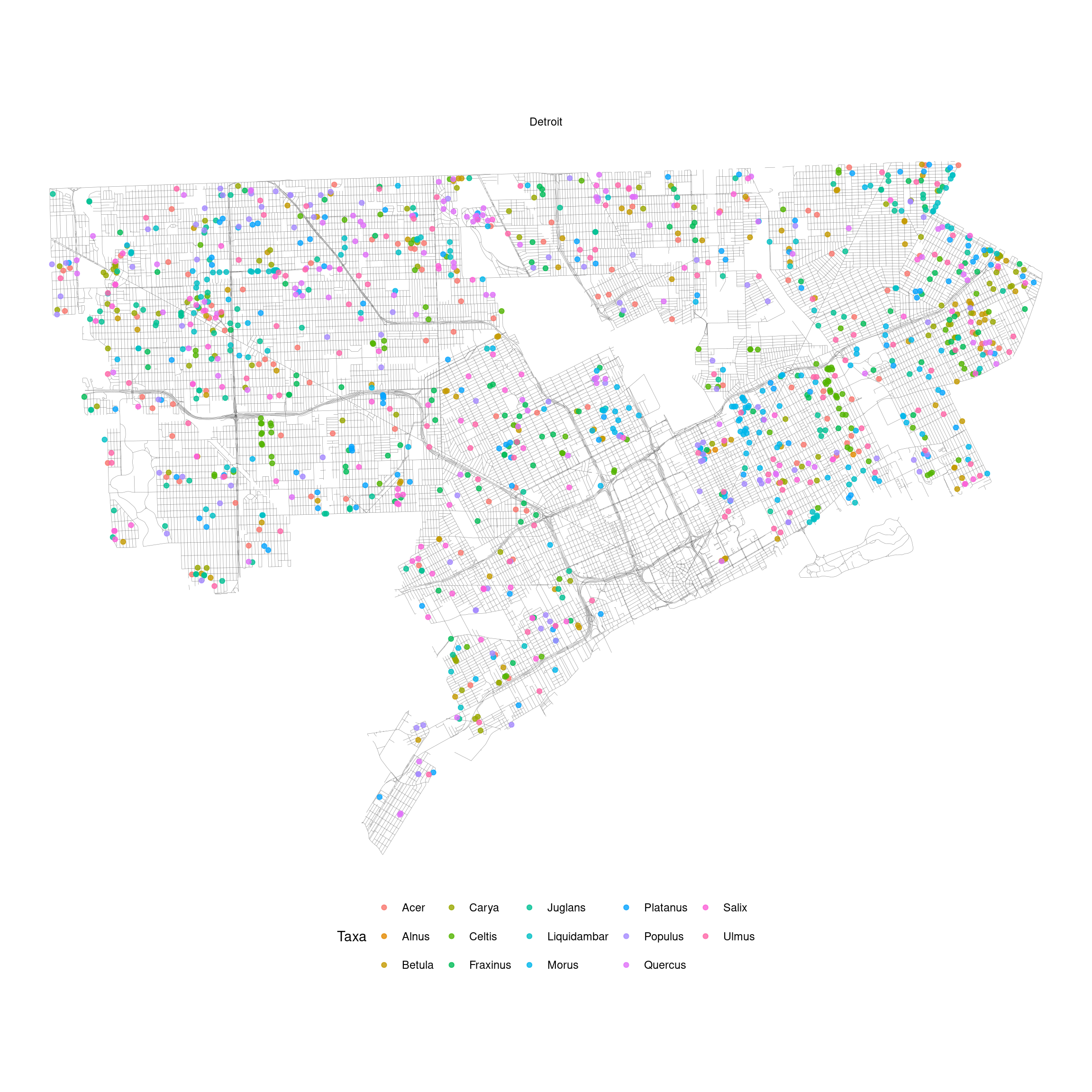
Map plant occurrence in a city.

source("code/data_occ_road_map.R")
p_plant_map

3.4 PlanetScope data

PlanetScope data were previously processed using batchplanet package.

Here we visualize a subset of street trees in Detroit overlayed on a true-color PlanetScope image on May 8, 2017.

source("code/data_ps_snap.R")
p_ps_snap

Pollen count and plant occurrence data. (A) Map of pollen counting stations associated with the National Allergy Bureau (NAB) and plant records near selected pollen counting stations. All pollen counting stations are marked in crossed circles, with ten selected stations in this study highlighted in red. Plant occurrence data from street tree inventory, land cover classification, and crowdsourcing are marked in blue points. (B) Pollen phenology of eleven key pollen-producing taxa in ten selected stations. (C) Spatial distribution of pollen-producing plants at ten study sites. Basemap show streets in cities. For simplicity, random 200 plants are visualized for each site.

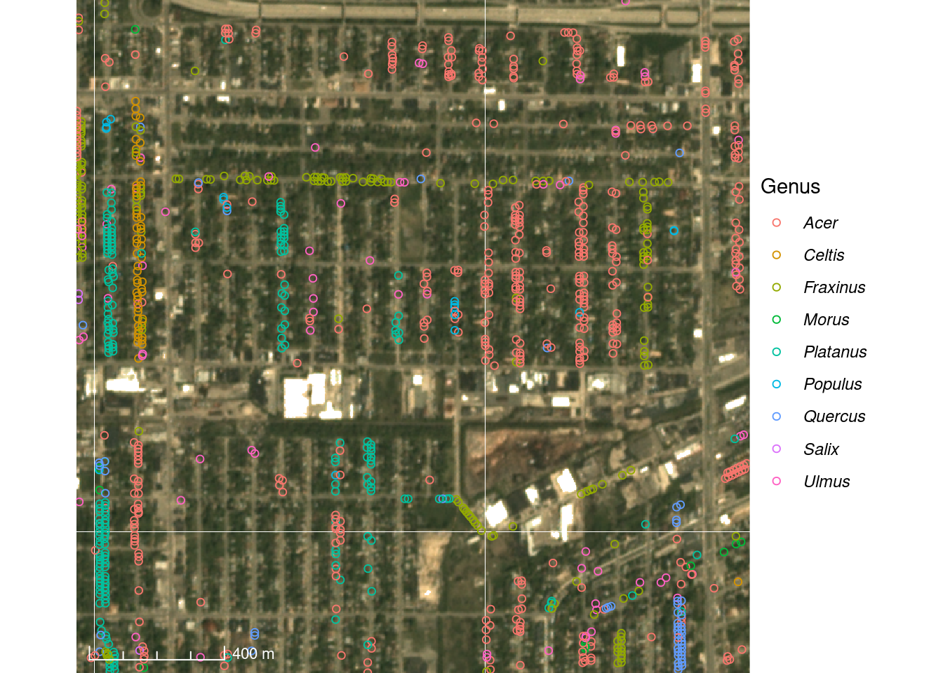
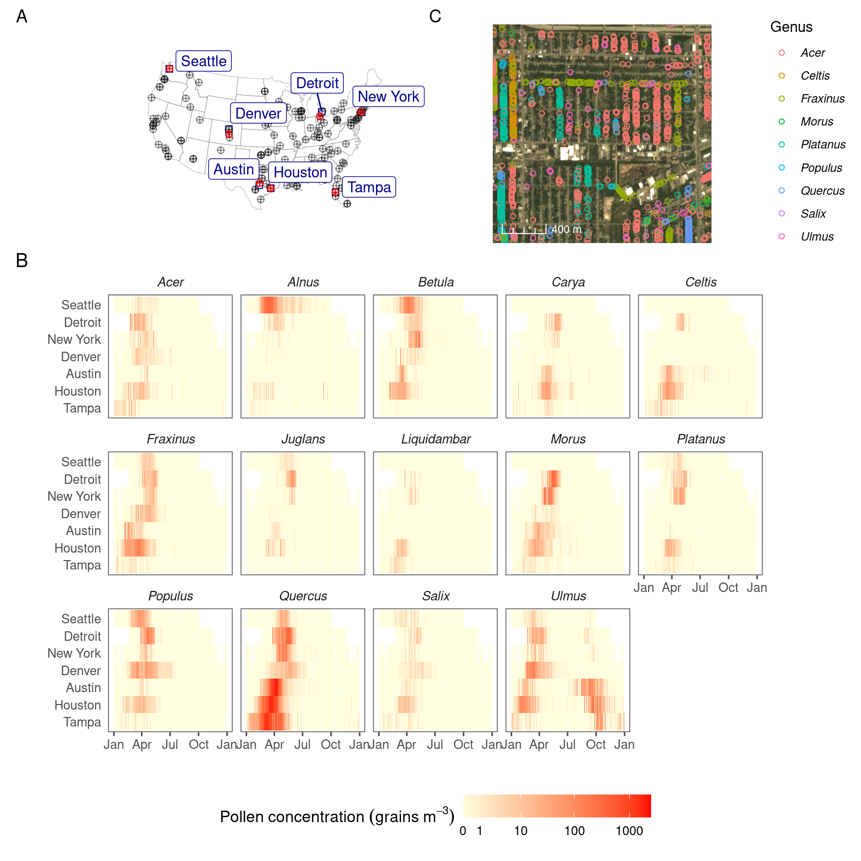
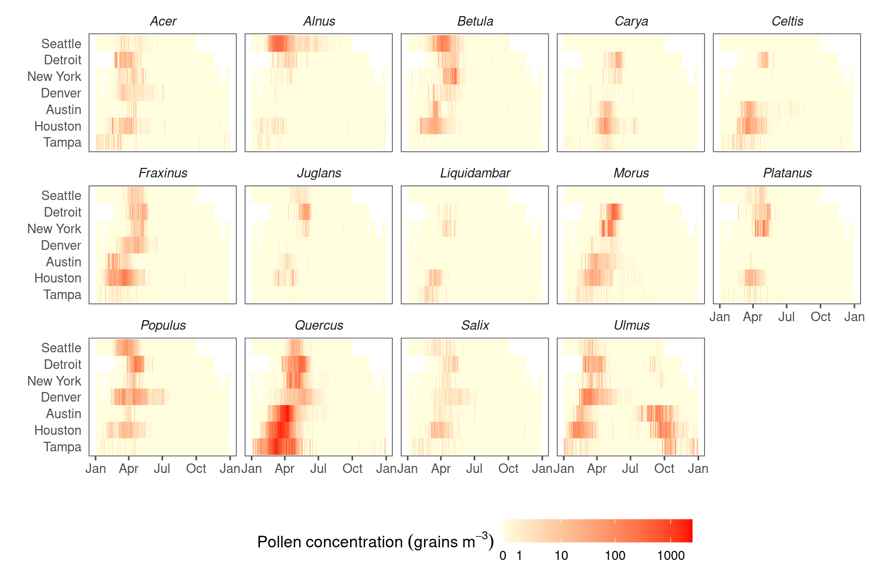
Figure 3.2: Pollen count and plant occurrence data. (A) Map of pollen counting stations associated with the National Allergy Bureau (NAB) and plant records near selected pollen counting stations. All pollen counting stations are marked in crossed circles, with ten selected stations in this study highlighted in red. Plant occurrence data from street tree inventory, land cover classification, and crowdsourcing are marked in blue points. (B) Pollen phenology of eleven key pollen-producing taxa in ten selected stations. (C) Spatial distribution of pollen-producing plants at ten study sites. Basemap show streets in cities. For simplicity, random 200 plants are visualized for each site.

3.5 Characterize phenology

Set green-up/down thresholds for each taxa.

source("code/city_prep.R")

Read in green-up down day of year previously processed using the batchplanet package.

source("code/city_doy.R")

Convert into probability density.

source("code/city_freq.R")

Process NAB and NPN data into probability density representing city-level flowering and pollen phenology, respectively.

source("code/city_data.R")

3.6 Tune parameters

Prepare some functions for plotting.

source("code/city_plot.R")

Tune green-up/down threshold and leaf-flower lag with NAB data.

source("code/city_tune.R")

3.7 Visualize predictions

Prepare for Shiny app by copying result figures to the current folder. Shiny app code is in ./shinyapp/app.R. Needs to deploy app once every time results are changed.

source("code/city_shiny.R")

Display results in a Shiny app.

Make some summary plots.

source("code/city_plot_subset.R")

p_comp_1city

p_comp_1taxa

p_comp_1taxa2city

p_city_corr

3.8 Cross validation

Plot correlation between mean annual temperature (MAT) and lag between green-up/down frequency and pollen count. * A positive lag means leafing phenology leads pollen phenology; a negative lag means leafing phenology lags pollen phenology.

source("code/city_clim_plot.R")
p_lag_clim

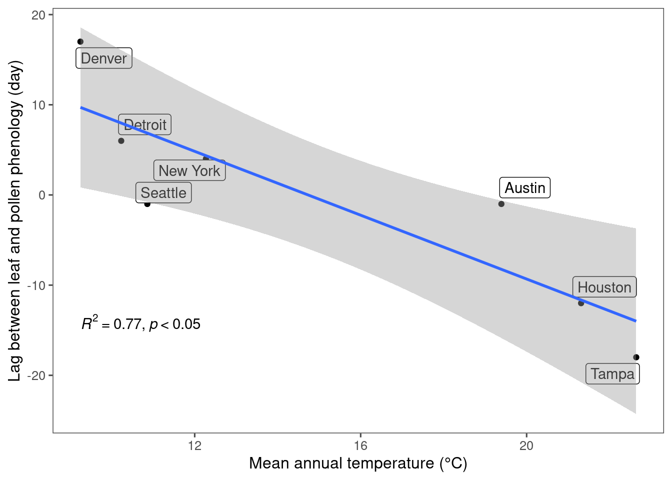* At warmer places, oak pollen tend to precede 50% green-up and vice versa.

Linear regression to check significance of the correlation.

source("code/city_clim_reg.R")
p_slope

We conducted leave-one-out cross validation to test the robustness of the climate-phenology relationship and the effectiveness of using it to infer flowering phenology in new locations. Specifically, we removed a random city from the pollen dataset at a time, matched leafing and pollen phenology in the other cities, and modeled the climate-lag correlation. We predicted the leafing-phenology lag with the linear model and subsequently predicted the flowering phenology from known leafing phenology at the city held for validation. We evaluated the accuracy of our methods by calculating the RMSE between the predicted flowering phenology and standardized pollen count observations at the cities held for validation.

source("code/city_loocv.R")

3.9 Evaluate performance

source("code/city_fit.R")

df_fit_all %>%
  drop_na(nrmse) %>%
  group_by(method) %>%
  summarise(
    median = median(nrmse),
    mean = mean(nrmse),
    lower = quantile(nrmse, 0.025),
    upper = quantile(nrmse, 0.975),
    n = n()
  )

## # A tibble: 2 × 6
##   method        median  mean  lower upper     n
##   <fct>          <dbl> <dbl>  <dbl> <dbl> <int>
## 1 in-sample      0.142 0.159 0.0881 0.336   282
## 2 out-of-sample  0.145 0.173 0.0982 0.360    33

df_fit_all %>%
  drop_na(nrmse) %>%
  filter(method == "in-sample") %>%
  group_by(taxa) %>%
  summarise(
    median = median(nrmse),
    mean = mean(nrmse),
    lower = quantile(nrmse, 0.025),
    upper = quantile(nrmse, 0.975),
    n = n()
  ) %>%
  arrange(desc(median))

## # A tibble: 15 × 6
##    taxa        median  mean  lower upper     n
##    <chr>        <dbl> <dbl>  <dbl> <dbl> <int>
##  1 Alnus        0.190 0.172 0.107  0.239    13
##  2 Acer         0.189 0.214 0.100  0.408    23
##  3 Ulmus early  0.172 0.203 0.111  0.435    28
##  4 Betula       0.157 0.154 0.0971 0.207    23
##  5 Salix        0.156 0.156 0.0947 0.242    19
##  6 Morus        0.144 0.148 0.0832 0.244    22
##  7 Platanus     0.142 0.147 0.0853 0.241    18
##  8 Populus      0.141 0.142 0.0972 0.215    23
##  9 Fraxinus     0.140 0.149 0.0912 0.248    20
## 10 Juglans      0.140 0.143 0.109  0.204    15
## 11 Ulmus late   0.136 0.148 0.110  0.204    15
## 12 Quercus      0.135 0.154 0.0967 0.321    33
## 13 Carya        0.130 0.135 0.104  0.174    15
## 14 Celtis       0.124 0.130 0.0993 0.184    10
## 15 Liquidambar  0.110 0.110 0.0868 0.127     5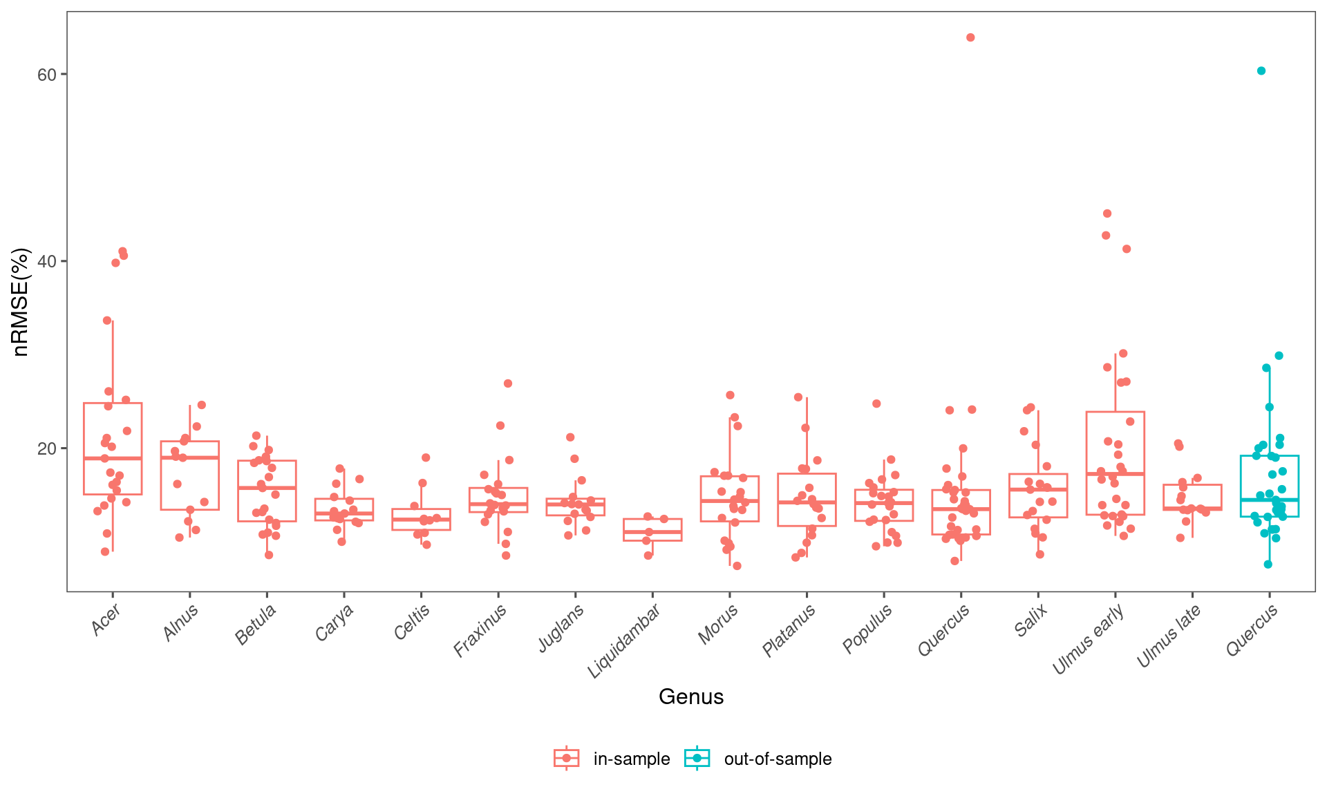

p_taxa_nrmse

df_fit_all %>%
  drop_na(spearman) %>%
  group_by(method) %>%
  summarise(
    median = median(spearman),
    mean = mean(spearman),
    lower = quantile(spearman, 0.025),
    upper = quantile(spearman, 0.975),
    n = n()
  )

## # A tibble: 2 × 6
##   method        median  mean lower upper     n
##   <fct>          <dbl> <dbl> <dbl> <dbl> <int>
## 1 in-sample      0.567 0.544 0.125 0.845   282
## 2 out-of-sample  0.691 0.679 0.337 0.910    33

df_fit_all %>%
  group_by(method, sig) %>%
  summarise(n = n())

## # A tibble: 3 × 3
## # Groups:   method [2]
##   method        sig                 n
##   <fct>         <chr>           <int>
## 1 in-sample     non-significant    16
## 2 in-sample     significant       266
## 3 out-of-sample significant        33

df_fit_all %>%
  drop_na(spearman) %>%
  filter(method == "in-sample") %>%
  group_by(taxa) %>%
  summarise(
    median = median(spearman),
    mean = mean(spearman),
    lower = quantile(spearman, 0.025),
    upper = quantile(spearman, 0.975),
    n = n()
  ) %>%
  arrange(desc(median))

## # A tibble: 15 × 6
##    taxa        median  mean   lower upper     n
##    <chr>        <dbl> <dbl>   <dbl> <dbl> <int>
##  1 Quercus      0.751 0.733  0.491  0.918    33
##  2 Populus      0.659 0.623  0.220  0.827    23
##  3 Morus        0.610 0.600  0.432  0.784    22
##  4 Celtis       0.599 0.580  0.280  0.761    10
##  5 Ulmus early  0.590 0.542  0.145  0.834    28
##  6 Carya        0.575 0.590  0.421  0.750    15
##  7 Betula       0.557 0.537  0.127  0.814    23
##  8 Fraxinus     0.544 0.534  0.142  0.825    20
##  9 Ulmus late   0.544 0.477  0.138  0.678    15
## 10 Liquidambar  0.542 0.492  0.241  0.627     5
## 11 Acer         0.514 0.479  0.131  0.736    23
## 12 Alnus        0.500 0.427 -0.0246 0.785    13
## 13 Salix        0.468 0.430  0.0784 0.708    19
## 14 Platanus     0.460 0.460  0.125  0.719    18
## 15 Juglans      0.454 0.423  0.260  0.531    15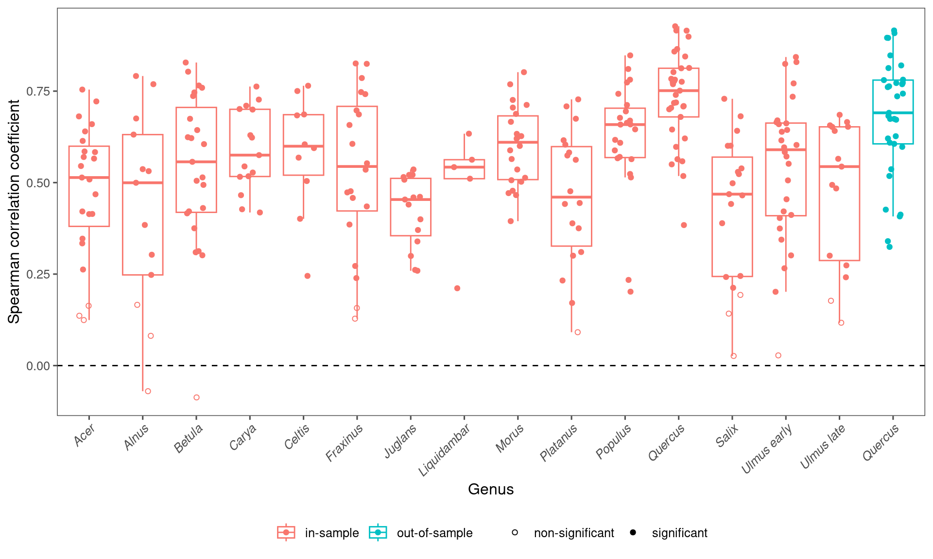

p_taxa_spearman

Validate with NPN instead of NAB and visualize.

df_fit_all %>%
  drop_na(spearman_npn) %>%
  group_by(method) %>%
  summarise(
    median = median(spearman_npn),
    mean = mean(spearman_npn),
    lower = quantile(spearman_npn, 0.025),
    upper = quantile(spearman_npn, 0.975),
    n = n()
  )

## # A tibble: 2 × 6
##   method        median  mean   lower upper     n
##   <fct>          <dbl> <dbl>   <dbl> <dbl> <int>
## 1 in-sample      0.479 0.398 -0.297  0.795   130
## 2 out-of-sample  0.470 0.476  0.0214 0.788    27

df_fit_all %>%
  group_by(method, sig_npn) %>%
  summarise(n = n())

## # A tibble: 6 × 3
## # Groups:   method [2]
##   method        sig_npn             n
##   <fct>         <chr>           <int>
## 1 in-sample     non-significant    35
## 2 in-sample     significant        95
## 3 in-sample     <NA>              152
## 4 out-of-sample non-significant     5
## 5 out-of-sample significant        22
## 6 out-of-sample <NA>                6

df_fit_all %>%
  drop_na(spearman_npn) %>%
  filter(method == "in-sample") %>%
  group_by(taxa) %>%
  summarise(
    median = median(spearman_npn),
    mean = mean(spearman_npn),
    lower = quantile(spearman_npn, 0.025),
    upper = quantile(spearman_npn, 0.975),
    n = n()
  ) %>%
  arrange(desc(median))

## # A tibble: 12 × 6
##    taxa        median  mean      lower upper     n
##    <chr>        <dbl> <dbl>      <dbl> <dbl> <int>
##  1 Acer         0.583 0.515 -0.0364    0.809    20
##  2 Juglans      0.576 0.524  0.195     0.671     6
##  3 Carya        0.556 0.319 -0.291     0.714    10
##  4 Quercus      0.542 0.503  0.0000180 0.820    27
##  5 Betula       0.515 0.367 -0.305     0.759    14
##  6 Celtis       0.444 0.444  0.306     0.582     2
##  7 Populus      0.387 0.415  0.156     0.677    14
##  8 Ulmus early  0.368 0.249 -0.601     0.790    18
##  9 Alnus        0.352 0.398  0.300     0.576     4
## 10 Platanus     0.276 0.207 -0.232     0.489     8
## 11 Fraxinus     0.246 0.232 -0.0995    0.550     3
## 12 Salix        0.242 0.300  0.0371    0.664     4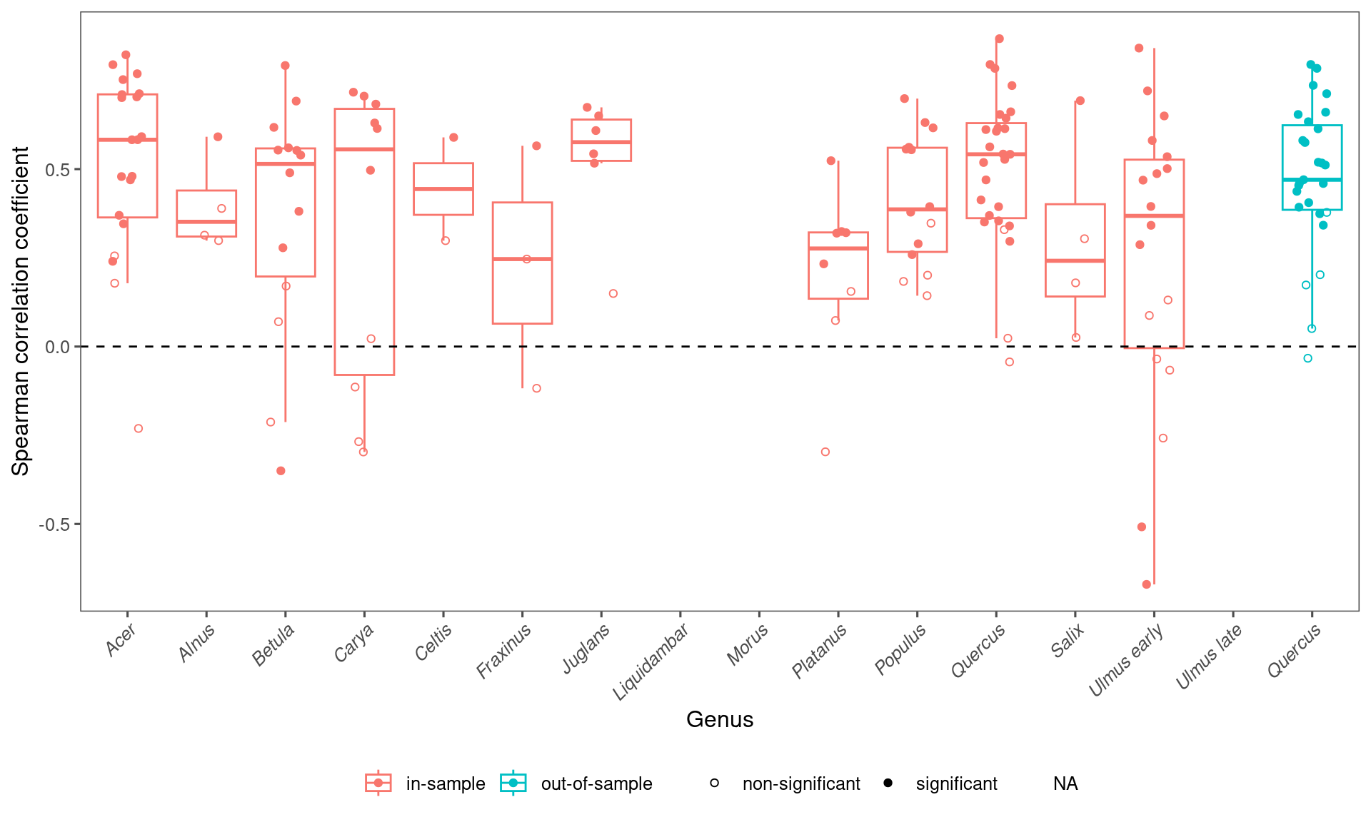

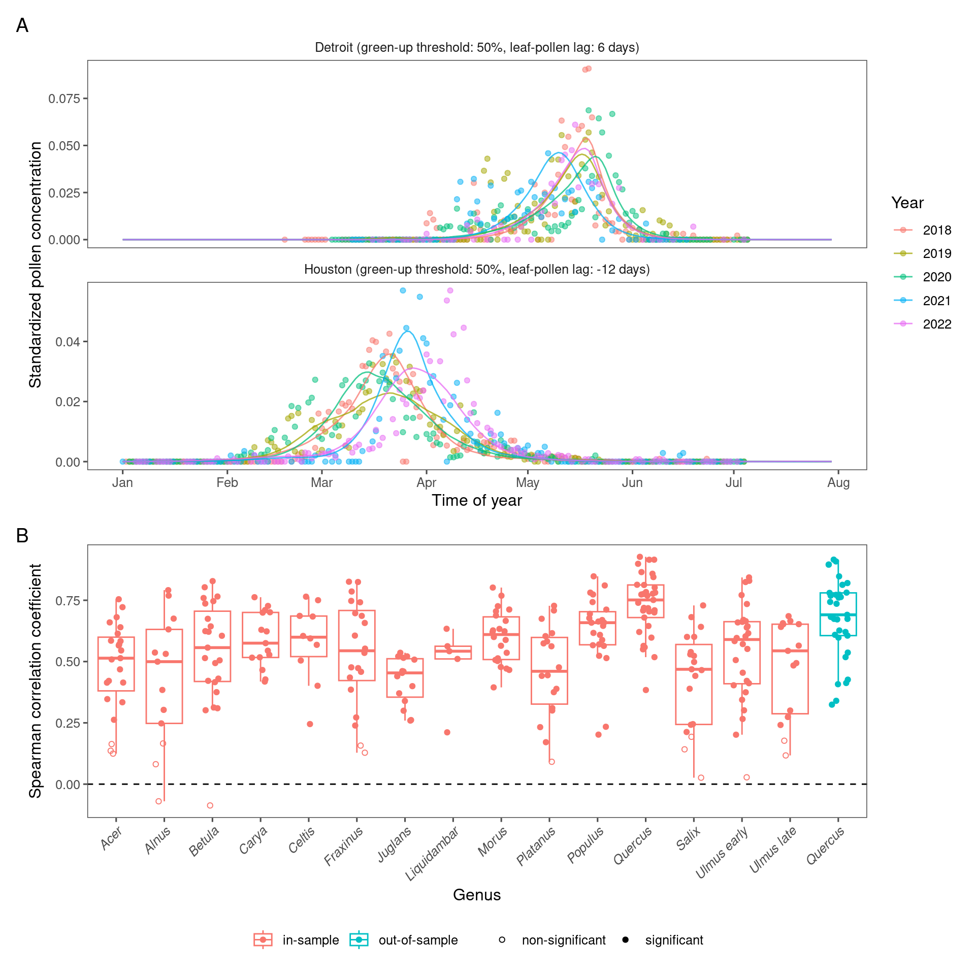
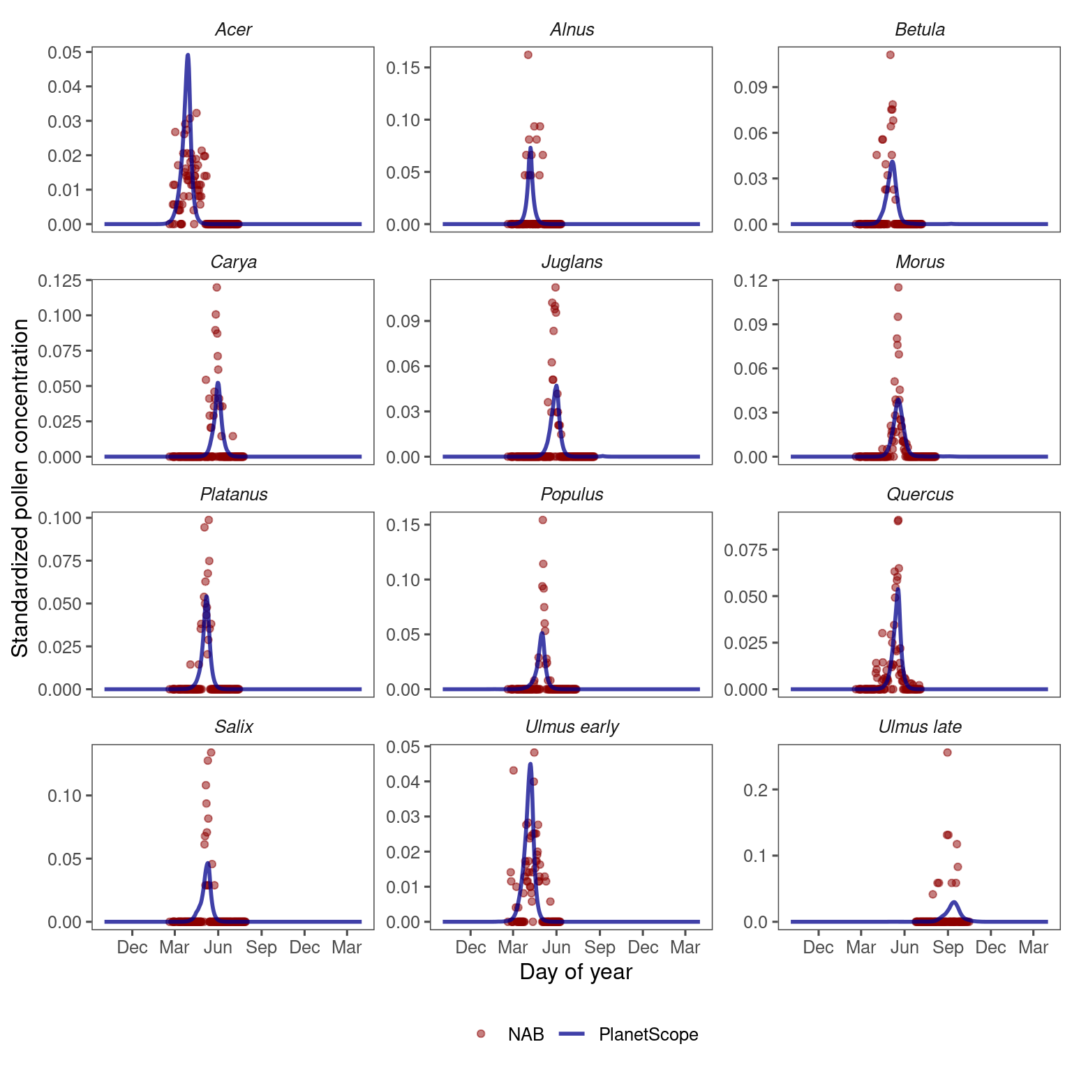
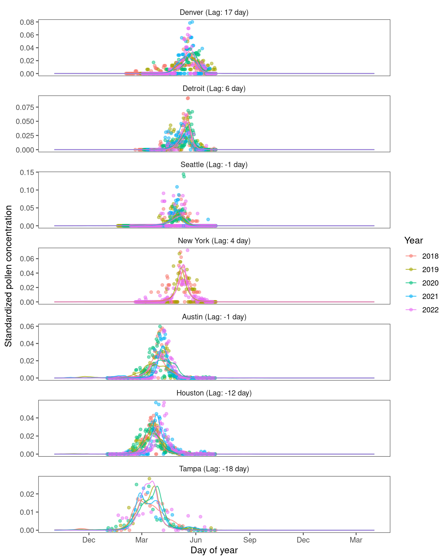
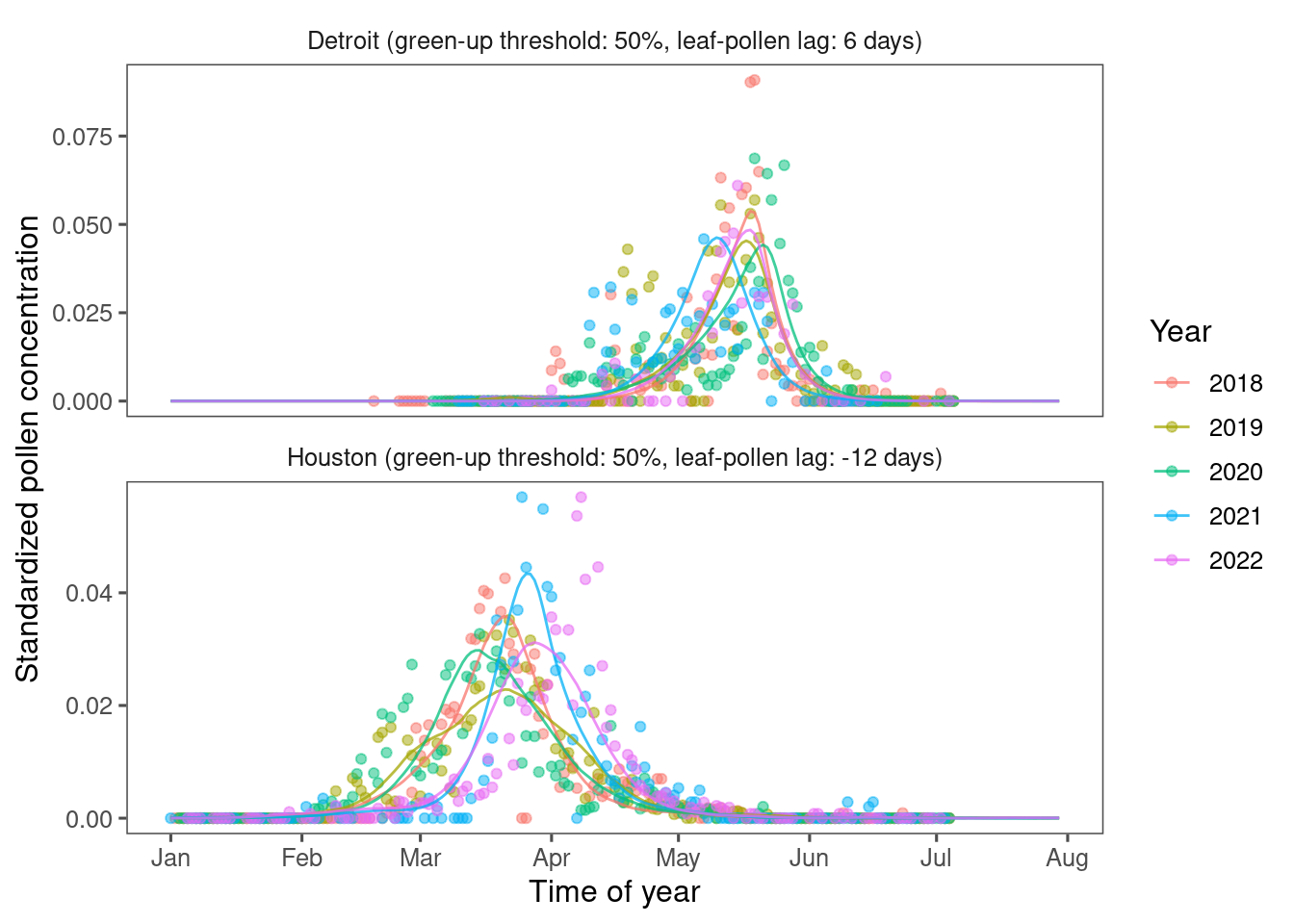
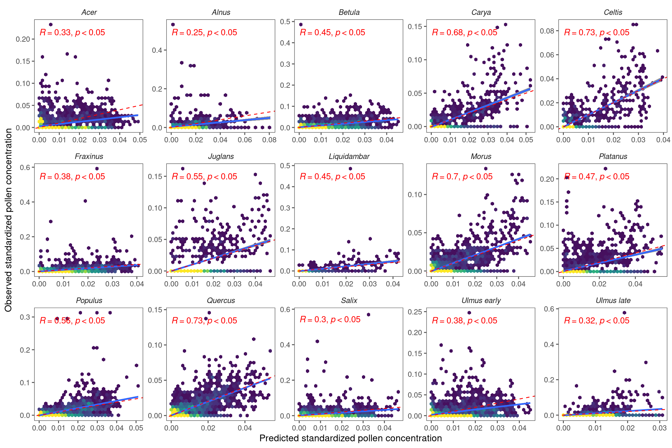
p_taxa_spearman_npn

Comparing remotely-sensed pollen phenology from PlanetScope and site-level pollen phenology from aerial sampling. (A) Pollen phenology inferred from remotely-sensed leafing phenology tuned to the optimal green-up/down thresholds and leafing-pollen lags (lines) compared to pollen phenology inferred from airborne pollen concentration (points). Pollen phenology from both data sources was converted to probability density within each site year for comparison. Here we show examples of oak (_Quercus_ spp.) pollen phenology at two sites on the south (Houston) and north (Detroit) of CONUS. (B) Accuracy of inferring pollen phenology across taxa measured with Spearman correlation coefficient, in-sample (fitting model with data from all sites) and out-of-sample (leave-one-out cross-validation).

Figure 3.3: Comparing remotely-sensed pollen phenology from PlanetScope and site-level pollen phenology from aerial sampling. (A) Pollen phenology inferred from remotely-sensed leafing phenology tuned to the optimal green-up/down thresholds and leafing-pollen lags (lines) compared to pollen phenology inferred from airborne pollen concentration (points). Pollen phenology from both data sources was converted to probability density within each site year for comparison. Here we show examples of oak (Quercus spp.) pollen phenology at two sites on the south (Houston) and north (Detroit) of CONUS. (B) Accuracy of inferring pollen phenology across taxa measured with Spearman correlation coefficient, in-sample (fitting model with data from all sites) and out-of-sample (leave-one-out cross-validation).