3.8 Model diagnostics and multicollinearity
As we saw in Section 3.3, checking the assumptions of the multiple linear model through the data scatterplots becomes tricky even when \(k=2\). To solve this issue, a series of diagnostic plots have been designed in order to evaluate graphically and in a simple way the validity of the assumptions. For illustration, we retake the wine dataset (download).
mod <- lm(Price ~ Age + AGST + HarvestRain + WinterRain, data = wine)We will focus only in three plots:
Residuals vs. fitted values plot. This plot serves mainly to check the linearity, although lack of homoscedasticity or independence can also be detected. Here is an example:
plot(mod, 1)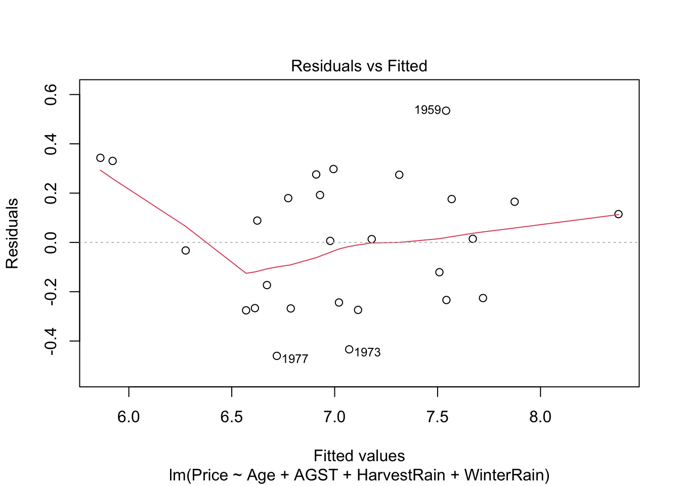
Under linearity, we expect the red line (a nonlinear fit of the mean of the residuals) to be almost flat. This means that the trend of \(Y_1,\ldots,Y_n\) is linear with respect to the predictors. Heteroskedasticity can be detected also in the form of irregular vertical dispersion around the red line. The dependence between residuals can be detected (harder) in the form of non randomly spread residuals.
QQ-plot. Checks the normality:
plot(mod, 2)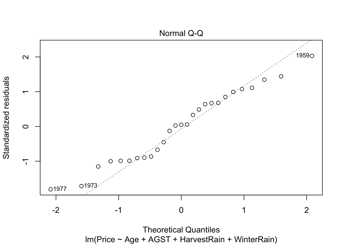
Under normality, we expect the points (sample quantiles of the standardized residuals vs. theoretical quantiles of a \(\mathcal{N}(0,1)\)) to align with the diagonal line, which represents the ideal position of the points if those were sampled from a \(\mathcal{N}(0,1)\). It is usual to have larger departures from the diagonal in the extremes than in the center, even under normality, although these departures are more clear if the data is non-normal.
Scale-location plot. Serves for checking the homoscedasticity. It is similar to the first diagnostic plot, but now with the residuals standardized and transformed by a square root (of the absolute value). This change transforms the task of spotting heteroskedasticity by looking into irregular vertical dispersion patterns into spotting for nonlinearities, which is somehow simpler.
plot(mod, 3)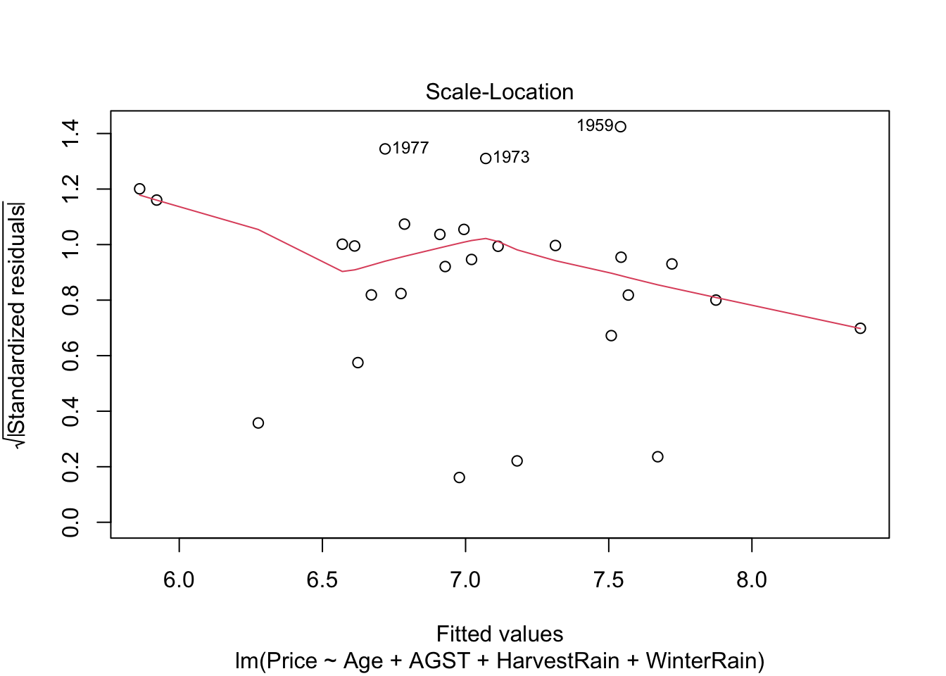
Under homoscedasticity, we expect the red line to be almost flat. If there are consistent nonlinear patterns, then there is evidence of heteroskedasticity.
If you type plot(mod), several diagnostic plots will be shown sequentially. In order to advance them, hit ‘Enter’ in the R console.
The next figures present datasets where the assumptions are satisfied and violated.
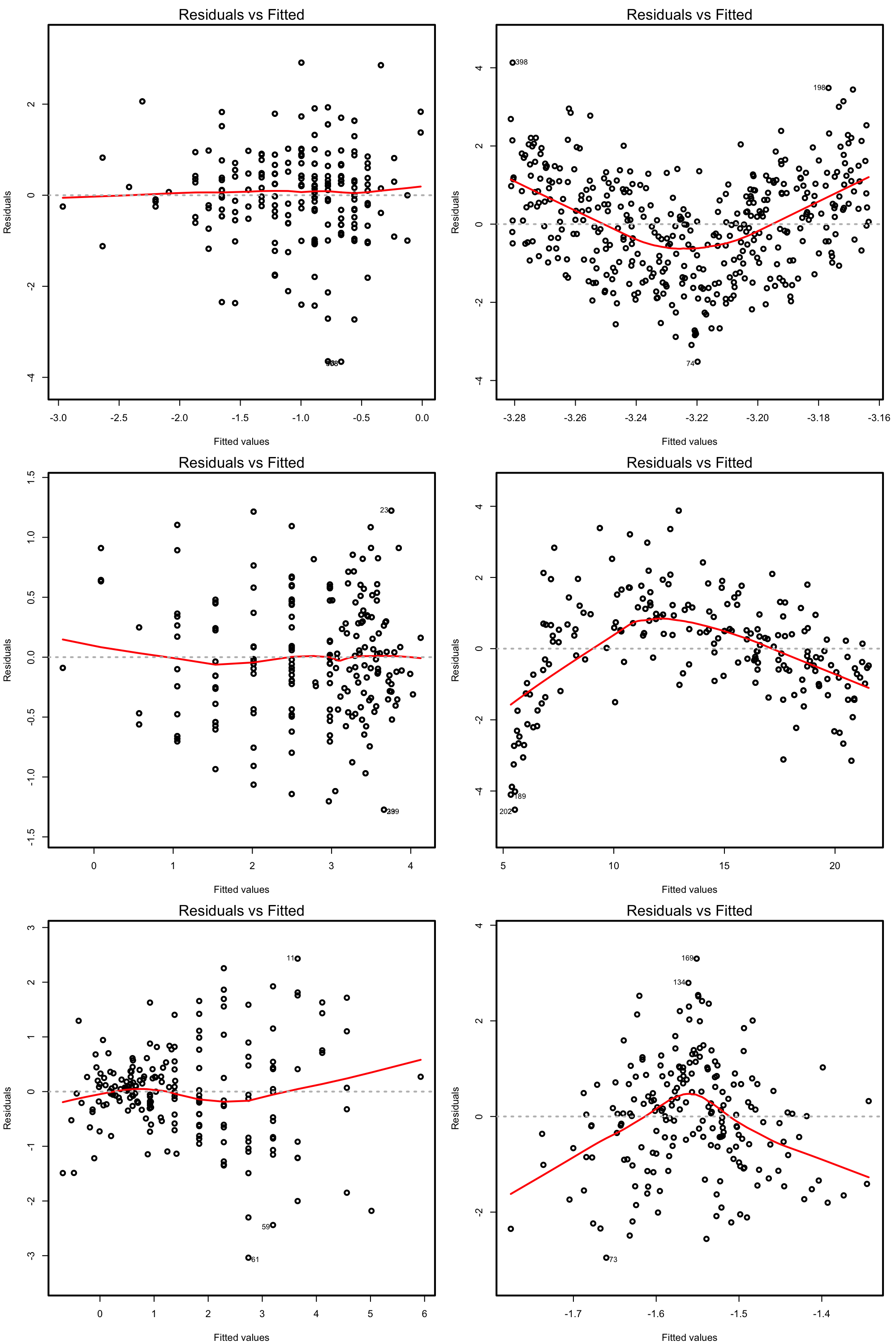
Figure 3.16: Residuals vs. fitted values plots for datasets respecting (left column) and violating (right column) the linearity assumption.
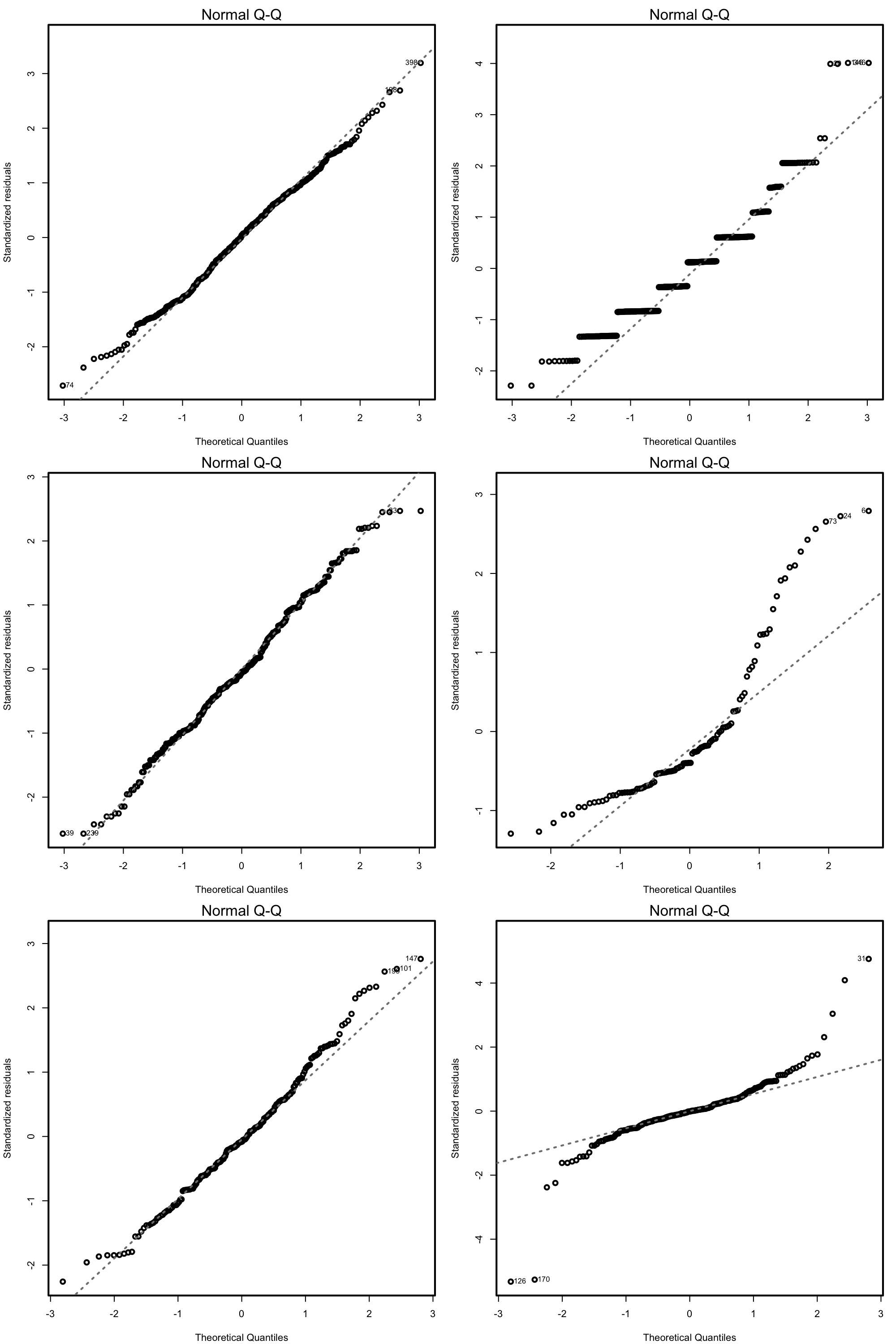
Figure 3.17: QQ-plots for datasets respecting (left column) and violating (right column) the normality assumption.
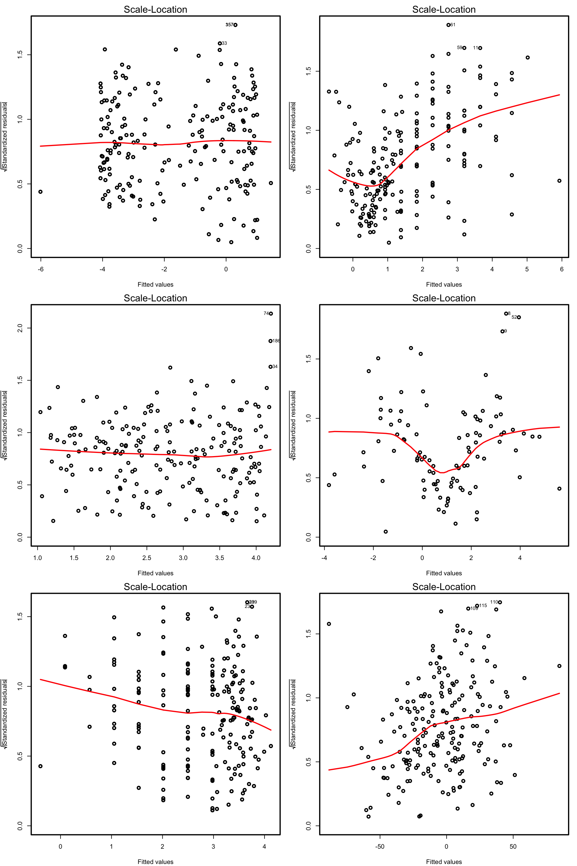
Figure 3.18: Scale-location plots for datasets respecting (left column) and violating (right column) the homoscedasticity assumption.
Load the dataset assumptions3D.RData(download) and compute the regressions y.3 ~ x1.3 + x2.3, y.4 ~ x1.4 + x2.4, y.5 ~ x1.5 + x2.5 and y.8 ~ x1.8 + x2.8. Use the three diagnostic plots to test the assumptions of the linear model.
A common problem that arises in multiple linear regression is multicollinearity. This is the situation when two or more predictors are highly linearly related between them. Multicollinearitiy has important effects on the fit of the model:
- It reduces the precision of the estimates. As a consequence, signs of fitted coefficients may be reversed and valuable predictors may appear as non significant.
- It is difficult to determine how each of the highly related predictors affects the response, since one masks the other. This may result in numerical instabilities.
An approach is to detect multicollinearity is to compute the correlation matrix between the predictors by cor (in R Commander: 'Statistics' -> 'Summaries' -> 'Correlation matrix...')
cor(wine)
##                  Price  WinterRain        AGST HarvestRain         Age
## Price        1.0000000  0.13488004  0.66752483 -0.50718463  0.46040873
## WinterRain   0.1348800  1.00000000 -0.32113230 -0.26798907 -0.05118354
## AGST         0.6675248 -0.32113230  1.00000000 -0.02708361  0.29488335
## HarvestRain -0.5071846 -0.26798907 -0.02708361  1.00000000  0.05884976
## Age          0.4604087 -0.05118354  0.29488335  0.05884976  1.00000000
## FrancePop   -0.4810720  0.02945091 -0.30126148 -0.03201463 -0.99227908
##               FrancePop
## Price       -0.48107195
## WinterRain   0.02945091
## AGST        -0.30126148
## HarvestRain -0.03201463
## Age         -0.99227908
## FrancePop    1.00000000
Here we can see what we already knew from Section 3.1.1, that Age and Year are perfectly linearly related and that Age and FrancePop are highly linearly related.
However, is not enough to inspect pair by pair correlations in order to get rid of multicollinearity. Here is a counterexample:
# Create predictors with multicollinearity: x4 depends on the rest
set.seed(45678)
x1 <- rnorm(100)
x2 <- 0.5 * x1 + rnorm(100)
x3 <- 0.5 * x2 + rnorm(100)
x4 <- -x1 + x2 + rnorm(100, sd = 0.25)

# Response
y <- 1 + 0.5 * x1 + 2 * x2 - 3 * x3 - x4 + rnorm(100)
data <- data.frame(x1 = x1, x2 = x2, x3 = x3, x4 = x4, y = y)

# Correlations - none seems suspicious
cor(data)
##            x1          x2         x3         x4           y
## x1  1.0000000  0.38254782  0.2142011 -0.5261464  0.31194689
## x2  0.3825478  1.00000000  0.5167341  0.5673174 -0.04428223
## x3  0.2142011  0.51673408  1.0000000  0.2500123 -0.77482655
## x4 -0.5261464  0.56731738  0.2500123  1.0000000 -0.28677304
## y   0.3119469 -0.04428223 -0.7748265 -0.2867730  1.00000000
A better approach is to compute the Variance Inflation Factor (VIF) of each coefficient \(\hat\beta_j\). This is a measure of how linearly dependent is \(X_j\) with the rest of predictors: \[ \text{VIF}(\hat\beta_j)=\frac{1}{1-R^2_{X_j|X_{-j}}} \] where \(R^2_{X_j|X_{-j}}\) is the \(R^2\) from a regression of \(X_j\) into the remaining predictors. The next rule of thumb gives direct insight into which predictors are multicollinear:
- VIF close to 1: absence of multicollinearity.
- VIF larger than 5 or 10: problematic amount of multicollinearity. Advised to remove the predictor with largest VIF.
VIF is called by vif and takes as argument a linear model (In R Commander: 'Models' -> 'Numerical diagnostics' -> 'Variance-inflation factors'). We continue with the previous example.
# Abnormal variance inflation factors: largest for x4, we remove it
modMultiCo <- lm(y ~ x1 + x2 + x3 + x4)
vif(modMultiCo)
##        x1        x2        x3        x4
## 26.361444 29.726498  1.416156 33.293983

# Without x4
modClean <- lm(y ~ x1 + x2 + x3)

# Comparison
summary(modMultiCo)
##
## Call:
## lm(formula = y ~ x1 + x2 + x3 + x4)
##
## Residuals:
##     Min      1Q  Median      3Q     Max
## -1.9762 -0.6663  0.1195  0.6217  2.5568
##
## Coefficients:
##             Estimate Std. Error t value Pr(>|t|)
## (Intercept)   1.0622     0.1034  10.270  < 2e-16 ***
## x1            0.9224     0.5512   1.673  0.09756 .
## x2            1.6399     0.5461   3.003  0.00342 **
## x3           -3.1652     0.1086 -29.158  < 2e-16 ***
## x4           -0.5292     0.5409  -0.978  0.33040
## ---
## Signif. codes:  0 '***' 0.001 '**' 0.01 '*' 0.05 '.' 0.1 ' ' 1
##
## Residual standard error: 1.028 on 95 degrees of freedom
## Multiple R-squared:  0.9144, Adjusted R-squared:  0.9108
## F-statistic: 253.7 on 4 and 95 DF,  p-value: < 2.2e-16
summary(modClean)
##
## Call:
## lm(formula = y ~ x1 + x2 + x3)
##
## Residuals:
##      Min       1Q   Median       3Q      Max
## -1.91297 -0.66622  0.07889  0.65819  2.62737
##
## Coefficients:
##             Estimate Std. Error t value Pr(>|t|)
## (Intercept)   1.0577     0.1033   10.24  < 2e-16 ***
## x1            1.4495     0.1162   12.47  < 2e-16 ***
## x2            1.1195     0.1237    9.05 1.63e-14 ***
## x3           -3.1450     0.1065  -29.52  < 2e-16 ***
## ---
## Signif. codes:  0 '***' 0.001 '**' 0.01 '*' 0.05 '.' 0.1 ' ' 1
##
## Residual standard error: 1.028 on 96 degrees of freedom
## Multiple R-squared:  0.9135, Adjusted R-squared:  0.9108
## F-statistic:   338 on 3 and 96 DF,  p-value: < 2.2e-16

# Variance inflation factors normal
vif(modClean)
##       x1       x2       x3
## 1.171942 1.525501 1.364878