2.4 Assumptions of the model
Why do we need assumptions? To make inference on the model parameters. In other words, to infer properties about the unknown population coefficients \(\beta_0\) and \(\beta_1\) from the sample \((X_1,Y_1),\ldots,(X_n,Y_n)\).

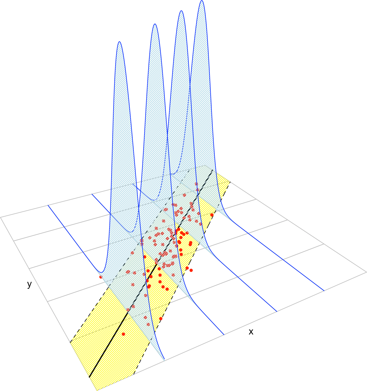
Figure 2.17: The key concepts of the simple linear model. The yellow band denotes where the \(95\%\) of the data is, according to the model.
The assumptions of the linear model are:
- Linearity: \(\mathbb{E}[Y|X=x]=\beta_0+\beta_1x\).
- Homoscedasticity: \(\mathbb{V}\text{ar}[\varepsilon_i]=\sigma^2\), with \(\sigma^2\) constant for \(i=1,\ldots,n\).
- Normality: \(\varepsilon_i\sim\mathcal{N}(0,\sigma^2)\) for \(i=1,\ldots,n\).
- Independence of the errors: \(\varepsilon_1,\ldots,\varepsilon_n\) are independent (or uncorrelated, \(\mathbb{E}[\varepsilon_i\varepsilon_j]=0\), \(i\neq j\), since they are assumed to be normal).
A good one-line summary of the linear model is (independence is assumed) \[\begin{align*} Y|X=x\sim \mathcal{N}(\beta_0+\beta_1x,\sigma^2) \end{align*}\]
Recall:
- Nothing is said about the distribution of \(X\). Indeed, \(X\) could be deterministic (called fixed design) or random (random design).
- The linear model assumes that \(Y\) is continuous due to the normality of the errors. However, \(X\) can be discrete!
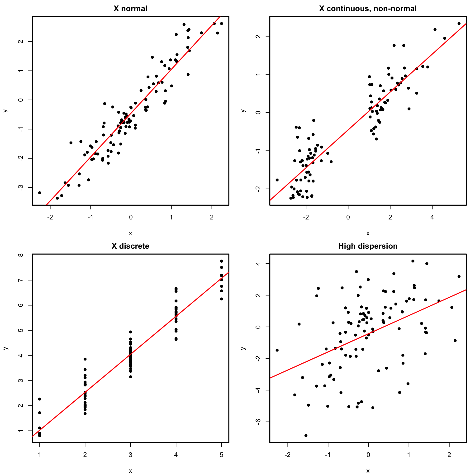
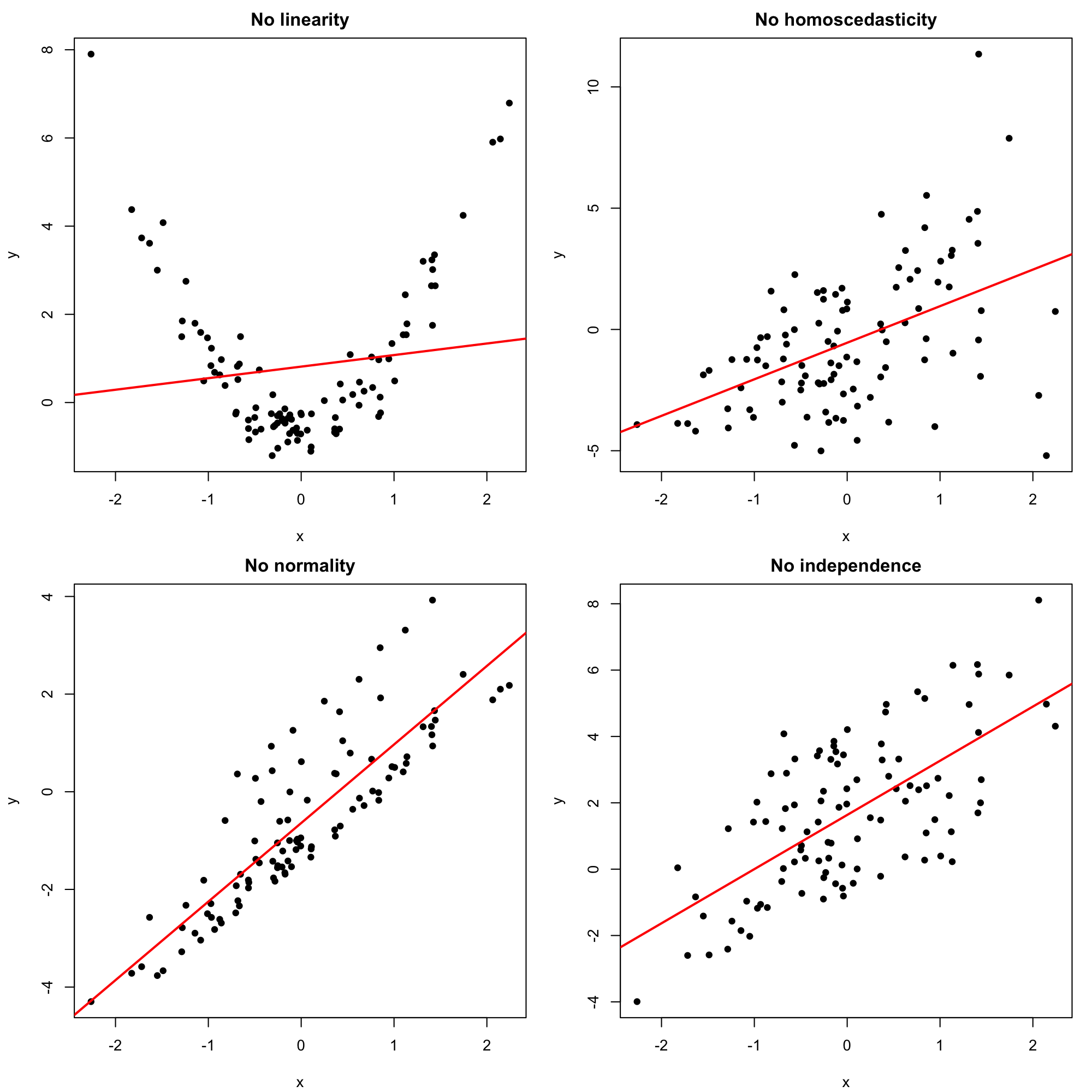
Figures 2.18 and 2.19 represent situations where the assumptions of the model are respected and violated, respectively. For the moment, we will focus on building the intuition for checking the assumptions visually. In Chapter 3 we will see more sophisticated methods for checking the assumptions. We will see also what are the possible fixes to the failure of assumptions.

Figure 2.18: Perfectly valid simple linear models (all the assumptions are verified).

Figure 2.19: Problematic simple linear models (a single assumption does not hold).
The dataset assumptions.RData (download) contains the variables x1, …, x9 and y1, …, y9. For each regression y1 ~ x1, …, y9 ~ x9:
- Check whether the assumptions of the linear model are being satisfied (make a scatterplot with a regression line).
- State which assumption(s) are violated and justify your answer.