4 Day 4 (January 30)
4.1 Announcements
Please upload a photo of the signature sheet to Canvas to get 2 magic extra credit points.
Please read (and re-read) Ch. 2 and 3 in BBM2L book.
Table of distributions in book
Activity 2 is posted
4.2 Example with differential equations
Motivating data example
url <- "https://www.dropbox.com/scl/fi/uokqouco07c44cder5vse/Butler-et-al.-Table-1.csv?rlkey=z37llt9dgvs59dw0ee8hnu7uq&dl=1"
df1 <- read.csv(url)
plot(df1$Winter, df1$N, typ = "b", xlab = "Year", ylab = "Population Size",
ylim = c(0, 300), lwd = 1.5, pch = "*")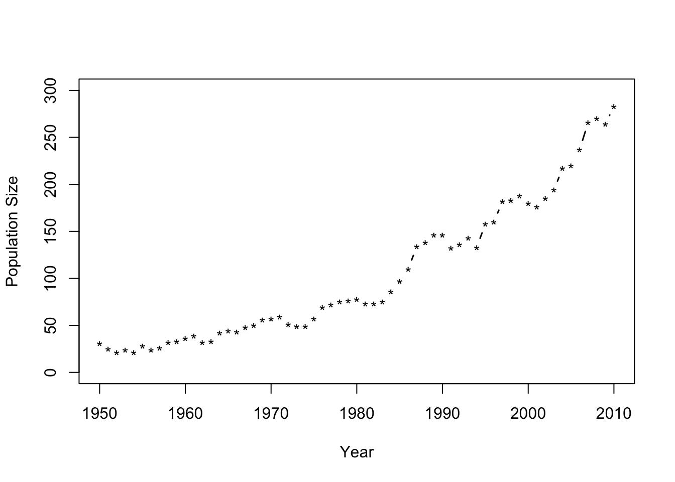
- Statistical model \[y_t\sim~\text{Poisson}(\lambda(t))\] where \[\lambda(t)=\lambda_{0}e^{\gamma(t-t_0)}\]
- Assume \(\lambda_0\) is known and equal to the the population size in 1950 (\(\lambda_0 = 31\))
- We want to obtain the distribtuion of \(\gamma\) given the data \(\mathbf{y}\)
- What else do we need to fully specify the model?
- Statistical model \[y_t\sim~\text{Poisson}(\lambda(t))\] where \[\lambda(t)=\lambda_{0}e^{\gamma(t-t_0)}\]
K <- 10^6                   # Number of samples to try
samples <- matrix(,K,2)     # Save samples
lambda0 <- df1$N[1]         # Lambda0
y <- df1$N[-1]              # Data
t <- df1$Winter[-1] - 1950  # Time

for(i in 1:K){

  gamma <- runif(1,0,0.1)
  lambda <- lambda0*exp(gamma*t)
  y.sample <- rpois(length(t),lambda)

  samples[i,1] <- mean(abs(y-y.sample))
  samples[i,2] <- gamma
}

par(mfrow=c(1,2))
hist(samples[,2],col="grey", main="Prior distribution",xlab=expression(gamma),ylab=expression("["*gamma*"]"),ylim=c(0,100),freq=FALSE,breaks=seq(0,0.1,by=0.005))
hist(samples[which(samples[,1]<30),2],ylim=c(0,100),xlim=range(samples[,2]),col="grey", main="Posterior distribution",xlab=expression(gamma*"|"*bold(y)),ylab=expression("["*gamma*"|"*bold(y)*"]"),freq=FALSE,breaks=seq(0,0.1,by=0.005)) 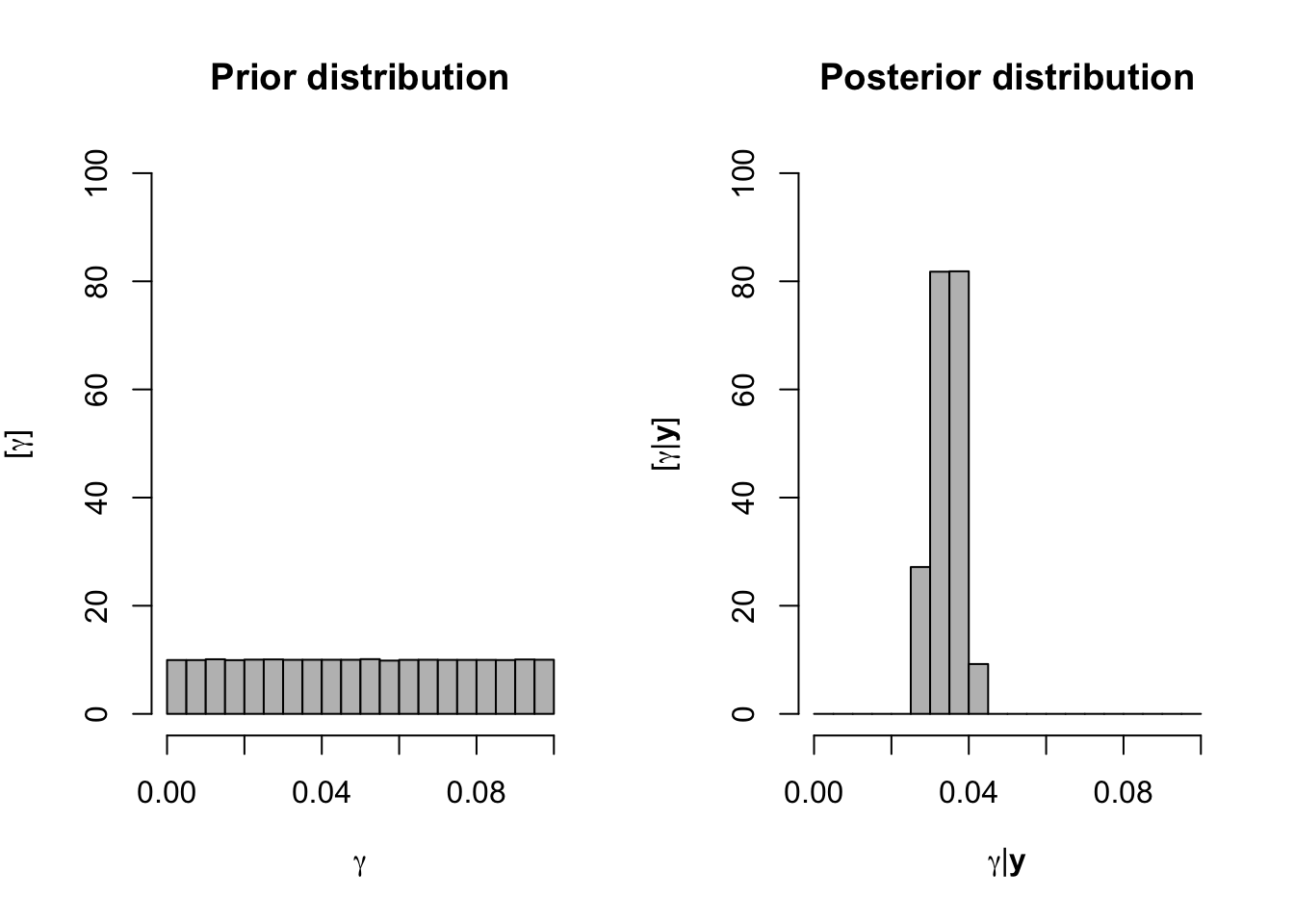
4.3 Building our first statistical model
- The backstory
- Building a statistical model using a likelihood-based (classical) approach
- Specify (write out) the likelihood
- Select an approach to estimate unknown parameters (e.g., maximum likelihood)
- Quantify uncertainty in unknown parameters (e.g., using normal approximation, see here)
- Building a statistical model using a Bayesian approach
- Specify (write out) the likelihood/data model
- Specify the parameter model (or prior) including hyper-parameters
- Select an approach to obtain the posterior distribution
- Analytically (i.e., pencil and paper)
- Simulation-based (e.g., Metropolis-Hastings, MCMC, importance sampling, ABC, etc)
4.4 Numerical Integration
Why do we need integrals to do Bayesian statistics?
- Example using Bayes theorem to estimate prevalence rate of rabies
- Why it is important to keep track of what we are calculating (i.e., clarity in what is being estimated)
Numerical approximation vs. analytical solutions
Definition of a definite integral \[\int_{a}^b f(z)dz = \lim_{Q\to\infty} \sum_{q=1}^{Q}\Delta q f(z_q)\] where \(\Delta q =\frac{b-a}{Q}\) and \(z_q = a + \frac{q}{2}\Delta q\).
Riemann approximation (midpoint rule)\[\int_{a}^b f(z)dz \approx \sum_{q=1}^{Q}\Delta q f(z_q)\] where \(\Delta q =\frac{b-a}{Q}\) and \(z_q = a + \frac{2q - 1}{2}\Delta q\).
Using similar approach in R (Adaptive quadrature)
## 0.9999367 with absolute error < 4.8e-12