21 Dynamic simulations

This chapter on dynamic simulations is an extension of the previous Chapter 20 on Basic simulations. Rather than using simple simulations that merely explicate a problem description, we now venture into the terrain of more dynamic ones. The term “dynamic” refers to the fact that we explicitly allow for changes in parameters and the constructs they represent. As these changes are typically incremental, our simulations will proceed in a step-wise fashion and store sequences of parameter values.

Conceptually, we distinguish between two broad types of systems and corresponding variables and dynamics: Changing agents and changing environments. This provides a first glimpse on the phenomenon of learning and on representing environmental uncertainty (in the form of multi-armed bandits with risky options). As both of these terms hint at a large and important family of models, we will only cover the general principles here.

Preparation

Recommended background readings for this chapter include:

• Chapter 2: Multi-armed Bandits of the book Reinforcement Learning: An Introduction by Sutton & Barto (2018). Related resources include:
  • Materials provided by Richard S. Sutton at incompleteideas.net (including the book’s PDF, data, code, figures, and slides)
  • A summary script of the introductory sections is available here
• Chapters 26 and 27 of Page (2018)

Preflections

• What are dynamics?

• What is the difference between an agent and its environment?

• Which aspects or elements of a simulation can be dynamic?

• What do we need to describe or measure to understand changes?

• How does this change the way in which we construct our simulations?

21.1 Introduction

Imagine a simple-minded organism that faces an unknown environment. The organism has a single need (e.g., find food) and a limited repertoire for action (e.g., move, eat, rest). To fulfill its solitary need, it navigates a barren and rugged surface that occasionally yields a meal, and may face a series of challenges (e.g., obstacles, weather conditions, and various potential dangers). Which cognitive and perceptual-motor capacities does this organism require to reach its goal and sustain itself? And which other aspects of the environment does its success depend on?

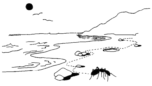
Figure 21.1: An ant foraging for food in an environment. (Image from this blog post.)

This example is modeled on a basic foraging scenario discussed by Simon (1956), but is reflected in many similar models that study how some organism (e.g., a simple robot) explores and exploits an initially unknown environment (e.g., a grid-world offering both rewards and risks).

Although this may be a toy scenario, it allows distilling some key elements that are required for addressing basic questions of rationality. For instance, the scenario is based on a conceptual distinction between an organism and its environment. As the organism can be simple or complex — think of an ant, a human being, or an entire organization — we will refer to it as an agent. Given some goal, the agent faces the problem of “behaving approximately rationally, or adaptively, in a particular environment” (Simon, 1956, p. 130).

The conceptual distinction between agent and its environment is helpful, but not as simple and straightforward as it seems. For instance, perceptions of environmental states, memories of past events, and cues or traces left by earlier explorations may all be important sources of information — but are these information sources part of the agent or of its environment? Researchers from artificial intelligence and the fields of embodied and distributed cognition have argued that the boundaries are blurred. Additionally, the status of the category labels “agent” vs. “environment” is a matter of perspective: From the perspective of any individual, all other agents are part of the environment.

Note two key challenges on elementary dimensions: Things can be unknown or uncertain. When things are unknown (or risky), we can discover them by exploring or familiarizing us with them. Doing so assumes some flexibility on part of the agent (typically described as acquiring knowledge or learning), but can lead to reliable estimates of the unknown parameters. By contrast, when things are uncertain (e.g., when options or rewards can change in unpredictable ways), even intimate familiarity does not provide reliable estimates or certainty for any particular moment. Thus, both ignorance and uncertainty are problematic, but uncertainty is the more fundamental problem.

Importantly, both problems are inevitable when things are dynamic (i.e., changing). The fact that changes tend to create both ignorance and uncertainty makes it essential that our models can accommodate changes. However, changes are not just a source of problems, but also part of the solution: When aspects of our environment change, processes of adaptation and learning allow us to adjust again. (Note that this may sound clever and profound, but is really quite simple: When things change, we need to change as well — and the reverse is also true.)

Simon addresses the distinction between optimizing and satisficing. Organisms typically adapt well-enough to meet their goals (i.e., satisfice), but often fail to optimize.

Clarify key terminology: What changes when things are dynamic?

• agents (goals, knowledge and beliefs, policies/strategies, capacities for action)

• environments (tasks, rewards, temporal and spatial structures)

• interactions between agents and environments

21.1.1 What is dynamic?

The term dynamics typically implies movement or changes.

By contrast, our simulations so far were static in two ways:

• the environment was fixed (even when being probabilistic): One-shot games, without dependencies between subsequent states.

• the range of actions was fixed a priori and behavioral policy of agents did not change)

Three distinct complicating aspects:

1. Environmental dependencies: Later states in the environment depend on earlier ones.

2. Learning: Behavior of agents (i.e., their repertoire or selection of actions) changes as a function of experience or time.

3. Interaction with agents: Environment or outcomes change as a function of (inter-)actions with agents.

Different types of dependencies (non-exhaustive):

• temporal dependencies: Later states depend on previous ones

• interactions: Interdependence between environment and an agent’s actions.

• types of learning: agents can change their behavioral repertoire (actions available) or policies (selection of actions) over time

If the environment changes as a function of its prior states and/or the actions of some agent(s), it cannot be simulated a priori and independently of them (i.e., without considering actions).

Typical programming elements:

• Trial-by-trial structure of simulations (i.e., using loops or tables that are filled incrementally). As agents or environments change over time, we need to explicitly represent time and typically proceed in a step-wise (i.e., iterative) fashion.
  For instance, an agent may interact with an environment over many decision cycles, observes an outcome, and adjusts its expectations or actions accordingly. Time is typically represented as individual steps \(t\) (aka. periods, rounds, or trials) that range from some starting value (e.g., 0 or 1) to some large number (e.g., \(n_T = 100\)). Often, we will even need inner loops within outer loops (e.g., for running several repetitions of a simulation, to assess the robustness of results).

• More abstract representations: For instance, rather than explicitly representing each option in an environment, we could simply use a vector of integers to represent a series of chosen options (i.e., leave the state of the environment implicit). Similarly, an agent’s beliefs regarding the reward quality of options may be represented as a vector of their choice probabilities.

Examples:

• Environments with some form of “memory” (e.g., planting corn or wheat, changes in crop cycle)

• Interactions: Environments that change by agent’s actions:

  • TRACS (environmental options change as function of agent’s actions) vs.
    
  • Tardast (dynamic changes over time and agent actions)

21.1.2 Topics and models addressed

In this chapter, we provide a glimpse on some important families of models, known as
learning agents and multi-armed bandits (MABs).

Typical topics addressed by these paradigms include: Learning by adjusting expectations to observed rewards and trade-off between exploration vs. exploitation.

Typical questions asked in these contexts include: How to learn to distinguish better from worse options? How to optimally allocate scarce resources (e.g., limitations of attention, experience, time)?

We can distinguish several levels of (potential) complexity:

1. Dynamic agents: Constant environment, but an agent’s beliefs or repertoire for action changes based on experience (i.e., learning agent).

2. Dynamic environments: Assuming some agent, the internal dynamics in the environment may change. MAB tasks with responsive or restless bandits (e.g., adding or removing options, changing rewards for options).

3. Benchmarking the performance of different strategies: Evaluating the interactions between an agent (with different strategies) and environments: Agent and/or environment depend on strategies and previous actions.

A further level of complexity will be addressed in the next chapter on Social situations (see Chapter 22): 4. Tasks involving multiple agents: Additional interactions between agents (e.g., opportunities for observing and influencing others, using social information, social learning, including topics of communication, competition, and cooperation, etc.).

21.1.3 Models of agents, environments, and interactions

The key motivation for dynamic simulations is that things that are alive constantly keep changing. Thus, our models need to allow for and capture changes on a variety of levels. The term “things” is used in its widest possible sense (i.e., entities, including objects and subjects), including environments, agents, representations of them, and their interactions.

General issues addressed here (separating different types of representations and tasks):

• Modeling an agent (e.g., internal states and overt actions)

• Modeling the environment (e.g., options, rewards, and their probabilities)

A mundane, but essential aspect: Adding data structures for keeping track of changes (in both agents or environments).

Note: When the term “dynamic” makes you think of video games and self-driving cars, the environments and problems considered here may seem slow and disappointing. However, we will quickly see that even relatively simple tasks can present plenty of conceptual and computational challenges.

Key goals and topics of this chapter:

• Implementing a basic model of learning (e.g., RL, Section 21.2)

• Implementing dynamic environments (e.g., with uncertain rewards, MAB, Section 21.3)

• Evaluating dynamic models (e.g., by benchmarking strategy performance, RTA, Section 21.4)

21.2 Models of learning

We first assume a stable environment and a dynamic agent. Adapting agents are typically described by the phenomenon of learning.

An elementary situation — known as binary forced choice — is the following: An agent faces a choice between several alternative options. For now, let’s assume that there are only two options and both options are deterministic and stable: Each option yields a constant reward by being chosen.

• How can the agent learn to choose the better option?

A general solution to the task of learning the best alternative is provided by reinforcement learning (RL, Sutton & Barto, 2018). The framework of RL assumes that intelligent behavior aims to reach goals in some environment. Organisms learn by exploring their environments in a trial-and-error fashion. As successful behavior is reinforced, their behavioral patterns is shaped by receiving and monitoring rewards. Some authors even assume that any form of natural or artifical intelligence (including perception, knowledge acquisition, language, logical reasoning, and social intelligence) can be understood as subserving the maximization of reward (Silver et al., 2021).

Although RL has developed into a core branch of machine learning and artificial intelligence, it is based on a fairly simple theory of classical conditioning (Rescorla & Wagner, 1972). In the following, we will illustrate its basic principles (following Page, 2018, p. 306f.).

Basic idea

Assume that an agent is facing a choice between \(N\) options with rewards \(\pi(1) ... \pi(N)\). The learner’s internal model or perspective on the world is represented as a set of weights \(w\) that denote the expected value of or preference for each of the available options (i.e., \(w(1) ... w(N)\)). Given this representation, successful learning consists in adjusting the values of these weights to the (stable) rewards of the environment and choosing options accordingly.

Learning proceeds in a stepwise fashion: In each step, the learner acts (i.e., chooses an option), observes a reward, and then adjusts the weight of the chosen option (i.e., her internal expectations or preferences). Formally, each choice cycle is characterized by two components:

1. Choosing: The probability of choosing \(k\)-th alternative is given by:

\[P(k) = \frac{w(k)}{\sum_{i}^{N} w(i)}\]

2. Learning: The learner adjusts the weight of the \(k\)-th alternative after choosing it and receiving its reward \(\pi(K)\) by adding the following increment:

\[\Delta w(k) = \alpha \cdot P(k) \cdot [\pi(k) - A]\]

with two parameters describing characteristics of the learner: \(\alpha > 0\) denoting the learning rate (aka. rate of adjustment or step size parameter) and \(A < \text{max}_{k}{\pi(k)}\) denoting the aspiration level.³²

Note the following details of the learning rule:

• The difference \([\pi(k) - A]\) is the reason for the \(\Delta\)-Symbol that commonly denotes differences or deviations. Here, we compare the observed reward \(\pi(k)\) to an aspiration level \(A\), which can be characterized as a measure of surprise: When a reward \(\pi(k)\) corresponds to our aspiration level \(A\), we are not surprised (i.e., \(\Delta w(k) = 0\)). By contrast, rewards much smaller or much larger than our aspirations are more surprising and lead to larger adjustments. If a reward value exceeds \(A\), \(w(k)\) increases; if it is below \(A\), \(w(k)\) decreases.

• The \(\Delta w(k)\)-increment specified by Page (2018) includes the current probability \(P(k)\) of choosing the \(k\)-th option as a weighting factor, but alternative formulations of \(\Delta\)-rules omit this factor or introduce additional parameters.

For details and historical references, see the Wikipedia pages to the Rescorla-Wagner model, Reinforcement learning and Q-learning. See Sutton & Barto (2018), for a general introduction to reinforcement learning.

Coding a model

To create a model that implements a basic learning agent that explores and adapts to a stable environment, we first define some objects and parameters:

# Initial setup (see Page, 2018, p. 308):

# Environment: 
alt <- c("A", "B")  # constant options
rew <- c(10, 20)    # constant rewards (A < B)

# Agent: 
alpha <- 1          # learning rate
A     <- 5          # aspiration level
wgt   <- c(50, 50)  # initial weights 

In the current model, the environmental options alt and their rewards rew are fixed and stable. Also, the learning rate alpha and A are assumed to be constants, but the weights wgt that represent the agent’s beliefs or expectations about the value of environmental options are parameters that may change after every cycle of choosing an action and observing a reward.

As the heart of our model, we translate functions 1. and 2. into R code:

# 1. Choosing an option: ------ 

p <- function(k){  # Probability of k:
  
  wgt[k]/sum(wgt)  # wgt denotes current weights
  
}

# Reward from choosing Option k: ------  

r <- function(k){
  
  rew[k]  # rew denotes current rewards
  
}

# 2. Learning: ------ 

delta_w <- function(k){  # adjusting the weight of k: 
  
  (alpha * p(k) * (r(k) - A))
  
}

Note that the additional function r(k) provides the reward obtained from choosing alternative k. Thus, r(k) is more a part of the environment than of the agent. Actually, it defines the interface between agent and environment. As the environmental rewards stored as rew are currently assumed to be constant, we could replace this function by writing rew[k] in the weight increment given by delta_w(k). However, as the r() function conceptually links the agent’s action (i.e., choosing option k) to the rewards provided by the environment rew and we will soon generalize this to stochastic environments (in Section 21.3), we already include this function here.³³

With these basic functions in place, we define an iterative loop for 1:n_T time steps t (aka. choice-reward cycles, periods, or rounds) to simulate the iterative process. In each step, we use p() to choose an action and delta_w() to interpret and adjust the observed reward:

# Environment: 
alt <- c("A", "B")  # constant options
rew <- c(10, 20)    # constant rewards (A < B)

# Agent: 
alpha <- 1          # learning rate
A     <- 5          # aspiration level
wgt   <- c(50, 50)  # initial weights 

# Simulation:
n_T <- 20  # time steps/cycles/rounds

for (t in 1:n_T){  # each step/trial: ---- 

  # (1) Use wgt to determine the current action: 
  cur_prob <- c(p(1), p(2))
  cur_act  <- sample(alt, size = 1, prob = cur_prob)
  ix_act   <- which(cur_act == alt)
  
  # (2) Update wgt (based on action & reward): 
  new_w <- wgt[ix_act] + delta_w(ix_act)  # increment weight by delta w
  wgt[ix_act] <- new_w  # update wgt
  
  # (+) User feedback:
  print(paste0(t, ": Choose ", cur_act, " (", ix_act, "), and ",
              "learn wgt = ", paste(round(wgt, 0), collapse = ":"), 
              " (A = ", A, ")"))
}

# Report result:
print(paste0("Final weight values (after ", n_T, " steps): ", 
             paste(round(wgt, 0), collapse = ":")))

Due to the use of sample() in selecting the current action cur_act (i.e., choosing either the 1st or 2nd option out of alt), running this code repeatedly will yield different results.

The repeated references to the weights wgt imply that this vector is a global variable that is initialized once and then accessed and changed at various points in our code (e.g., in p() and when updating the weights in the loop). If this should get problematic, we could pass wgt as an argument to every function.

Running this model yields the following output:

#> [1] "1: Choose A (1), and learn wgt = 52:50 (A = 5)"
#> [1] "2: Choose A (1), and learn wgt = 55:50 (A = 5)"
#> [1] "3: Choose B (2), and learn wgt = 55:57 (A = 5)"
#> [1] "4: Choose B (2), and learn wgt = 55:65 (A = 5)"
#> [1] "5: Choose B (2), and learn wgt = 55:73 (A = 5)"
#> [1] "6: Choose A (1), and learn wgt = 57:73 (A = 5)"
#> [1] "7: Choose B (2), and learn wgt = 57:81 (A = 5)"
#> [1] "8: Choose B (2), and learn wgt = 57:90 (A = 5)"
#> [1] "9: Choose B (2), and learn wgt = 57:99 (A = 5)"
#> [1] "10: Choose B (2), and learn wgt = 57:109 (A = 5)"
#> [1] "11: Choose A (1), and learn wgt = 59:109 (A = 5)"
#> [1] "12: Choose B (2), and learn wgt = 59:119 (A = 5)"
#> [1] "13: Choose A (1), and learn wgt = 61:119 (A = 5)"
#> [1] "14: Choose B (2), and learn wgt = 61:128 (A = 5)"
#> [1] "15: Choose B (2), and learn wgt = 61:139 (A = 5)"
#> [1] "16: Choose B (2), and learn wgt = 61:149 (A = 5)"
#> [1] "17: Choose A (1), and learn wgt = 62:149 (A = 5)"
#> [1] "18: Choose B (2), and learn wgt = 62:160 (A = 5)"
#> [1] "19: Choose B (2), and learn wgt = 62:170 (A = 5)"
#> [1] "20: Choose B (2), and learn wgt = 62:181 (A = 5)"
#> [1] "Final weight values (after 20 steps): 62:181"

The output is printed by the user feedback (i.e., the print() statements) that is provided at the end of each loop and after finishing its n_T cycles. Due to using sample() to determine the action (or option chosen) on each time step t, the results will differ every time the simulation is run.
Although we typically want to collect better records on the process, reading this output already hints at a successful reinforcement learning process: Due to the changing weights wgt, the better alternative (here: Option B) is increasingly preferred and chosen.

Practice

1. Which variable(s) allow us to see and evaluate that learning is taking place? What exactly do these represent (i.e., the agent’s internal state or overt behavior)? Why do we not monitor the values of cur_prob in each round?

2. Predict what happens when the reward value \(\pi(k)\) equals the aspiration level \(A\) (i.e., \(\pi(k) = A\)) or falls below it (i.e., \(\pi(k) < A\)). Test your predictions by running a corresponding model.

3. Playing with parameters:

   • Set n_T and alpha to various values and observe how this affects the rate and results of learning.

   • Set rew to alternative values on observe how this affects the rate and results of learning.

Keeping track

To evaluate simulations more systematically, we need to extend our model in two ways:

1. First, the code above only ran a single simulation of n_T steps. However, due to random fluctuations (e.g., in the results of the sample() function), we should not trust the results of any single simulation. Instead, we want to run and evaluate some larger number of simulations to get an idea about the variability and robustness of their results. This can easily be achieved by enclosing our entire simulation within another loop that runs several independent simulations.

2. Additionally, our initial simulation (above) used a print() statement to provide user feedback in each iteration of the loop. This allowed us to monitor the n_T time steps of our simulation and evaluate the learning process. However, displaying results as the model code is being executed becomes impractical when simulations get larger and run for longer periods of time. Thus, we need to collect required performance measures by setting up and using corresponding data structures as the simulation runs.

The following code takes care of both concerns: First, we embed our previous simulation within an outer loop for running a sequence of n_S simulations. Additionally, we prepare an auxiliary data frame data that allows recording the agent’s action and weights on each step (or choice-reward cycle) as we go along.

Note that working with two loops complicates setting up data (as its needs a total of n_S * n_T rows, as well as columns for the current values of s and t) and the indices for updating the current row of data. Also, using an outer loop that defines distinct simulations creates two possible levels for initializing information. In the present case, some information (e.g., the number of simulations, the number of steps per simulation, the available options, and their constant rewards) is initialized only once (globally). By contrast, we chose to initialize the parameters of the learner in every simulation (although we currently only update the weights wgt in each step).

The resulting simulation code is as follows:

# Simulation:
n_S <- 12  # Number of simulations     
n_T <- 20  # Number of time steps/cycles/rounds/trials (per simulation)

# Environmental constants: 
alt <- c("A", "B")  # constant options
rew <- c(10, 20)    # constant rewards (A < B)

# Prepare data structure for storing results: 
data <- as.data.frame(matrix(ncol = (3 + length(alt)), nrow = n_S * n_T))
names(data) <- c("s", "t", "act", paste0("w_", alt))

for (s in 1:n_S){     # each simulation: ---- 
  
  # Initialize agent: 
  alpha <- 1        # learning rate
  A <- 5            # aspiration level
  wgt <- c(50, 50)  # initial weights 
  
  for (t in 1:n_T){   # each step/trial: ---- 
    
    # (1) Use wgt to determine current action: 
    cur_prob <- c(p(1), p(2))
    cur_act <- sample(alt, size = 1, prob = cur_prob)
    ix_act <- which(cur_act == alt)
    
    # (2) Update wgt (based on reward): 
    new_w <- wgt[ix_act] + delta_w(ix_act)  # increment weight
    wgt[ix_act] <- new_w  # update wgt
    
    # (+) Record results:
    data[((s-1) * n_T) + t, ] <- c(s, t, ix_act, wgt)
    
  } # for t:n_T end.
  
  print(paste0("s = ", s, ": Ran ", n_T, " steps, wgt = ", 
               paste(round(wgt, 0), collapse = ":")))
  
} # for i:n_S end.
#> [1] "s = 1: Ran 20 steps, wgt = 66:167"
#> [1] "s = 2: Ran 20 steps, wgt = 68:156"
#> [1] "s = 3: Ran 20 steps, wgt = 61:184"
#> [1] "s = 4: Ran 20 steps, wgt = 83:96"
#> [1] "s = 5: Ran 20 steps, wgt = 63:180"
#> [1] "s = 6: Ran 20 steps, wgt = 63:171"
#> [1] "s = 7: Ran 20 steps, wgt = 67:156"
#> [1] "s = 8: Ran 20 steps, wgt = 57:209"
#> [1] "s = 9: Ran 20 steps, wgt = 61:192"
#> [1] "s = 10: Ran 20 steps, wgt = 62:173"
#> [1] "s = 11: Ran 20 steps, wgt = 61:183"
#> [1] "s = 12: Ran 20 steps, wgt = 73:126"

# Report result:
print(paste0("Finished running ", n_S, " simulations (see 'data' for results)"))
#> [1] "Finished running 12 simulations (see 'data' for results)"

The user feedback within the inner loop was now replaced by storing the current values of parameters of interest into a row of data. Thus, data collected information on all intermediate states:

Table 21.1: A record of simulation states and results.

s	t	act	w_A	w_B
1	1	1	52.50000	50.00000
1	2	1	55.06098	50.00000
1	3	1	57.68141	50.00000
1	4	2	57.68141	56.96499
1	5	2	57.68141	64.41812
1	6	1	60.04347	64.41812

Note that both the construction of our model and the selection of variables stored in data determine the scope of results that we can examine later. For instance, the current model did not explicitly represent the reward values received on every trial. As they were constant for each option, we did not need to know them here, but this may change if the environment became more dynamic (see Section 21.3). Similarly, we chose not to store the current value of the agent’s aspiration level \(A\) for every trial. However, if \(A\) ever changed within a simulation, we may want to store a record of its values in data.

Visualizing results

This allows us to visualize the learning process and progress. Figure 21.2 shows which option was chosen in each time step and simulation:

# Visualize results:
ggplot(data, aes(x = t)) + 
  facet_wrap(~s) + 
  geom_path(aes(y = act), col = Grau) + 
  geom_point(aes(y = act, col = factor(act)), size = 2) + 
  scale_color_manual(values = usecol(c(Bordeaux, Seegruen))) + 
  scale_y_continuous(breaks = 1:2, labels = alt) +  
  labs(title = paste0("Agent actions (choices) in ", n_S, " simulations"), 
       x = "Time steps", y = "Action", color = "Option:") + 
  theme_ds4psy()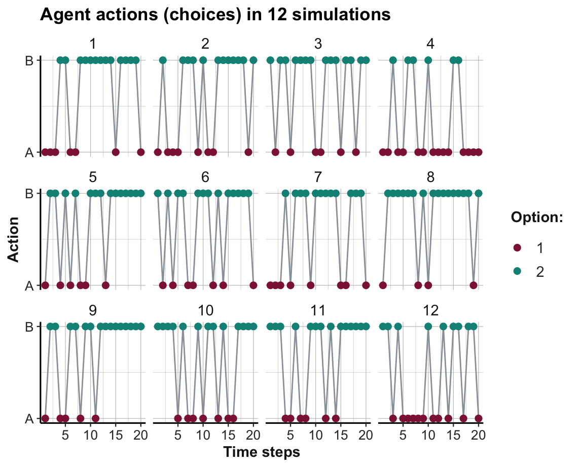

Figure 21.2: The agent’s action (i.e., option chosen) in a stable environment per time step and simulation.

As Option B yields higher rewards than Option A, learning would be reflected in Figure 21.2 by an increasing preference of B over A. Figure 21.3 shows the trends in option weights per time step for all 12 simulations:

ggplot(data, aes(x = t, group = s)) + 
  geom_path(aes(y = w_A), size = .5, col = usecol(Bordeaux, alpha = .5)) + 
  geom_path(aes(y = w_B), size = .5, col = usecol(Seegruen, alpha = .5)) + 
  labs(title = paste0("Agent weights (expectations/preferences) in ", n_S, " simulations"),   
       x = "Time steps", y = "Weights") + 
  theme_ds4psy()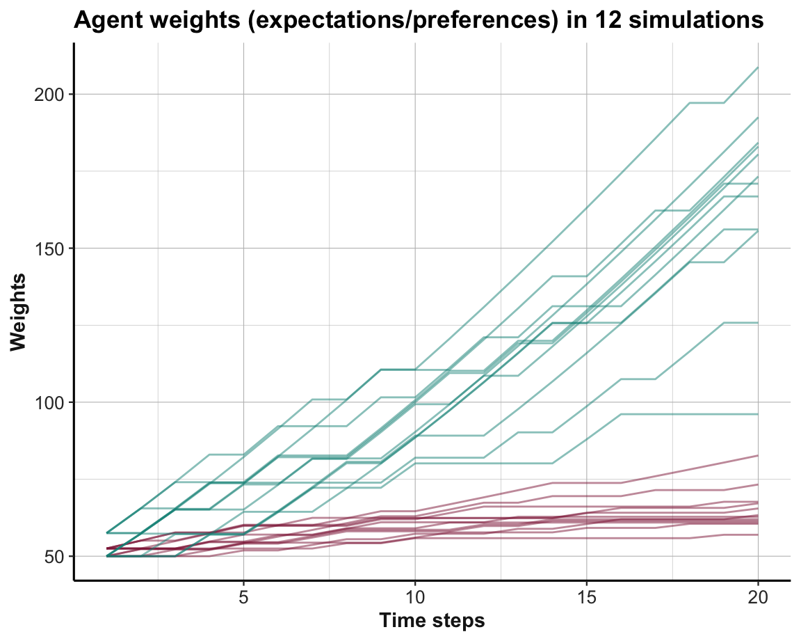

Figure 21.3: Trends in option weights in a stable environment per time step for all simulations.

The systematic difference in trends can be emphasized by showing their averages (Figure 21.4):

ggplot(data, aes(x = t)) + 
  geom_smooth(aes(y = w_A), size = 1, col = usecol(Bordeaux, alpha = .5)) + 
  geom_smooth(aes(y = w_B), size = 1, col = usecol(Seegruen, alpha = .5)) +
  labs(title = paste0("Trends in (average) agent weights in ", n_S, " simulations"),   
       x = "Time steps", y = "Weights", col = "Option:") + 
  theme_ds4psy()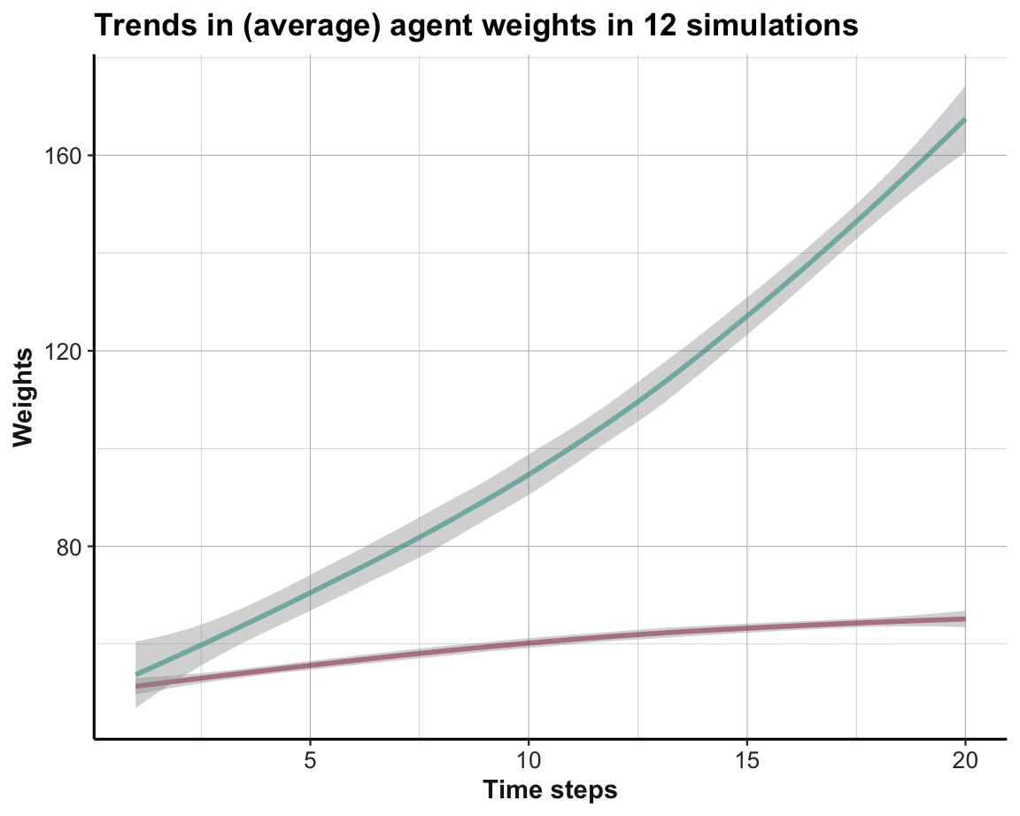

Figure 21.4: Average trends in option weights in a stable environment per time step for all simulations.

Interpretation

• The visualization of agent actions (in Figure 21.2) shows that most agents gradually chose the superior Option B more frequently. Thus, learning took place and manifested itself in a systematic trend in the choice behavior of the agent (particularly in later trials t).

• The visualization of agent weights (in Figure 21.3) illustrates that most learners preferred the superior Option B (shown in green) within about 5–10 trials of the simulation.

• The systematic preference of Option B over Option A (from Trial 5 onward) is further emphasized by comparing average trends (in Figure 21.4).

When interpreting the results of models, we must not forget that they show different facets of the same process. As the value of the weights wgt determine the probabilities of choosing each option (via p()), there is a logical link between the concepts illustrated by these visualizations: The behavioral choices shown in Figure 21.2 are a consequence of the weights shown in Figure 21.3 and 21.4, with some added noise due to random sampling. Thus, the three visualizations show how learning manifests itself on different conceptual and behavioral levels.

Practice

As both options always perform above the constant aspiration level (of \(A = 5\)), the weigth values wgt could only increase when experiencing rewards (as \(\Delta w > 0\)).

1. What would happen if the aspiration level was set to a value between both options (e.g., \(A = 15\))?

2. What would happen if the aspiration level was set to the value of the lower option (e.g., \(A = 10\))?

Boundary conditions

Reflecting on the consequences of different aspiration values highlights some boundary conditions that need to hold for learning to take place. We can easily see the impact of an aspiration level \(A\) matching the value of a current reward \(r(k)\).
Due to a lack of surprise (i.e., no difference \(r(k) - A = 0\)), the value of \(\Delta w(k)\) would become 0 as well. And if the value of \(A\) exceeds \(r(k)\), the difference \(r(k) - A\) and \(\Delta w(k)\) are negative, which leads to a reduction of the corresponding weight. If option weights were not bounded to be \(\geq 0\), this could create a problem for their conversion into a probability by \(p(k)\). However, as we chose a value \(A\) that was smaller than the smallest reward (\(A < min(\pi)\)), this problem could not occur here.

To avoid that all weights converge to zero, the value of the aspiration level \(A\) must generally be lower than the reward of at least one option (Page, 2018, p. 307). Under this condition, the two functions specified above (i.e., p() and w()) will eventually place almost all weight on the best alternative (as its weight always increases by the most). And using these weights for choosing alternatives implies that — in the long run — the best alternative will be selected almost exclusively.

Adapting aspirations

The basic framework shown here can be extended in many directions. For instance, the following example is provided by Page (2018) (p. 308). We consider two changes:

1. Endogeneous aspirations: Rather than using a constant aspiration level \(A\), a learner could adjust the value of \(A\) based on experience by setting it equal to the average reward value.

2. Fixed choice sequence: Rather than randomly sampling the chosen option (according to Equation 1, i.e., the probabilities of p()), we may want to evaluate the effects of a fixed sequence of actions (e.g., choosing B, B, A, B).

Given this setup, the question “What is being learned?” can only refer to the adjusted weights wgt (as the sequence of actions is predetermined). However, when moving away from a constant aspiration level, we also want to monitor the values of our adjusted aspiration level \(A_{t}\).

These changes can easily be implemented as follows:³⁴

# 1. Choosing: 
p <- function(k){  # Probability of k:
  
  wgt[k]/sum(wgt)  # wgt denotes current weights
  
}

# Reward from choosing k: 
r <- function(k){
  
  rew[k]  # rew denotes current rewards
  
}

# 2. REDUCED learning rule: 
delta_w <- function(k){ # Adjusting the weight of k: 
  
  # (alpha * p(k) * (r(k) - A))
  
  (alpha * 1 * (r(k) - A))  # HACK: seems to be assumed in Page (2018), p. 308
  
}

# Environment: 
alt <- c("A", "B")  # constant options
rew <- c(20, 10)    # constant rewards (A > B)
wgt <- c(50, 50)    # initial weights 

actions <- c("B", "B", "A", "B")
# actions <- rep("A", 10)
# actions <- rep(c("A", "B"), 50)

# Agent: 
alpha <- 1  # learning rate
A <- 5      # initial aspiration level

# Simulation:
n_T <- length(actions)  # time steps/rounds
r_hist <- rep(NA, n_T)  # history of rewards 

for (t in 1:n_T){

  # (1) Use wgt to determine current action: 
  # cur_prob <- c(p(1), p(2))
  # cur_prob <- c(1, 1)  # HACK: seems to be assumed in Page (2018), p. 308
  # cur_act <- sample(alt, size = 1, prob = cur_prob)
  cur_act <- actions[t]
  ix_act  <- which(cur_act == alt)
  
  # (2) Update wgt (based on reward): 
  new_w <- wgt[ix_act] + delta_w(ix_act)  # increment weight
  wgt[ix_act] <- new_w  # update wgt
  
  # (3) Determine reward and adjust aspiration level:
  r_hist[t] <- r(ix_act)           # store reward value in history 
  A <- mean(r_hist, na.rm = TRUE)  # adapt A  
  
  # (+) User feedback:
  print(paste0(t, ": ", cur_act, " (", ix_act, "), ", 
               "wgt = ", paste(round(wgt, 0), collapse = ":"), 
               ", A(", t, ") = ", round(A, 1)))
}
#> [1] "1: B (2), wgt = 50:55, A(1) = 10"
#> [1] "2: B (2), wgt = 50:55, A(2) = 10"
#> [1] "3: A (1), wgt = 60:55, A(3) = 13.3"
#> [1] "4: B (2), wgt = 60:52, A(4) = 12.5"

Practice

Let’s further reflect on the consequences of our endogeneous aspiration level \(A_{k}\):

1. How would \(A_{k}\) change when an agent chose one option for 10-times in a row?

2. How would \(A_{k}\) change when an agent alternated between Option A and Option B 50 times in a row (i.e., for a total of 100 trials)?

Limitations

Given the simplicity of our basic learning paradigm, we should note some limitations:

• Learning only from experience: As our model only learns from experienced options, it lacks the ability to learn from counterfactual information.

• Individual learning: The model here only considers an individual agent. Thus, it does not cover social situations and the corresponding phenomena of social information, social influence, and social learning.

• The model’s level of analysis is flexible or unclear: Some model may aim to represent the actual mechanism (implementation, e.g., in neuronal structures) while another may be content to be an abstract description of required components (e.g., a trade-off between hypothetical parts or processes).

Most of these limitations can be addressed by adding new elements to our basic learning paradigm. However, some limitations could also be interpreted as strengths: The simple, abstract and explicit nature of the model makes it easy to test and verify the necessary and sufficient conditions under which learning can take place. This higher degree of identifiability is the hallmark of formal models and distinguishes them from a verbal theory.

21.3 Dynamic environments

Our discussion so far allowed for some flexibility in an agent. Evidence for adaptive adjustments in the agent’s internal state or behavior surfaced as evidence for learning, but the environment was assumed to be stable. In reality, however, environments are rarely stable. Instead, a variety of possible changes keep presenting new challenges to a learning agent.

21.3.1 Multi-armed bandits (MABs)

A seemingly simple and subtle step away from a stable environment consists in adding uncertainty to the rewards received from choosing options. Adding uncertainty to the rewards of options can be achieved by rendering their rewards probabilistic (aka. stochastic). This creates a large and important family of models that are collectively known as multi-armed bandit (MAB) problems. The term “bandit” refers to a slot machine in a casino that allows players to continuously spend and occasionally win large amounts of money. As these bandits typically have only one lever, the term “multi-arm” refers to the fact that we can choose between several options (see Figure 21.5).

Figure 21.5: Three slot machines create a 3-armed bandit with uncertain payoffs for each option.

As all options are initially unfamiliar and may have different properties, an agent must first explore an option to estimate its potential rewards. With increasing experience, an attentive learner may notice differences between options and develop corresponding preferences. As soon as one option is perceived to be better than another, the agent must decide whether to keep exploring alternatives or to exploit the option that currently appears to be the best. Thus, MAB problems require a characteristic trade-off between exploration (i.e., searching for the best option) and exploitation (i.e., choosing the option that appears to be the best). The trade-off occurs because the total number of games (steps or trials) is finite (e.g., due to limitations of money or time). Thus, any trial spent on exploring an inferior option is costly, as it incurs a foregone payoff and reduces the total sum of rewards. Avoiding foregone payoffs creates a pressure towards exploiting seemingly superior options. However, we can easily imagine situations in which a better option is overlooked — either because the agent has not yet experienced or recognized its true potential or because an option has improved. Thus, as long as there remains some uncertainty about the current setup, the conflict between exploration and exploitation remains and must be negotiated.

MAB problems are widely used in biology, economics, engineering, psychology, and machine learning (see Hills et al., 2015, for a review). The main reason for this is that a large number of real-world problems can be mapped to the MAB template. For instance, many situations that involve a repeated choice between options (e.g., products, leisure activities, or even partners) or strategies (e.g., for advertising, developing, or selling stuff) can be modeled as MABs. Whereas the application contents and the mechanisms that govern the payoff distributions differ between tasks, the basic structure of a dynamic agent repeatedly interacting with a dynamic environment is similar in a large variety of situations. Thus, MAB problems provide an abstract modeling framework that accommodates many different tasks and domains.

Despite many parallels, different scientific disciplines still address different questions within the MAB framework. A basic difference consists in the distinction between theoretical vs. empirical approaches. As MABs offer a high level of flexibility, while still being analytically tractable, researchers in applied statistics, economics, operation research and decision sciences typically evaluate the performance of specific algorithms and aim for formal proofs of their optimality or boundary conditions. By contrast, researchers from biology, behavioral economics, and psychology are typically less concerned with optimality, and primarily interested in empirical data that informs about the strategies and rates of success when humans and other animals face environments that can be modeled as MABs. As both approaches are informative and not mutually exclusive, researchers typically need to balance the formal rigor and empirical relevance of their analysis — which can be described as a scientist facing a 2-armed bandit problem.

In the following, we extend our basic learning model by adding a MAB environment with probabilistic rewards. Chapter 2 of Reinforcement Learning: An Introduction by Sutton & Barto (2018) provides a more comprehensive introduction to MABs and corresponding models.

Basic idea

Assume that an agent is facing a choice between \(N\) options that yield rewards \(\pi(1) ... \pi(N)\) with some probability. In its simplest form, each option either yields a fixed reward (1) or no reward (0), but the probability of receiving a reward from each option is based on an unknown probability distribution \(p(1) ... p(N)\). More generally, an option \(k\) can yield a range of possible reward values \(\pi(k)\) that are given by a corresponding probability distribution \(p(k)\). As the rewards from such options can be analytically modeled by Bernoulli distributions, MAB problems with these properties are also called Bernoulli bandits (e.g., Page, 2018, p. 320). However, many other reward distributions and mechanisms for MABs are possible.

An agent’s goal in a MAB problem is typically to earn as much rewards as possible (i.e., maximize rewards). But as we mentioned above, maximizing rewards requires balancing the two conflicting goals of exploring options to learn more about them vs. exploiting known options for as much as possible. As exploring options can yield benefits (e.g., due to discovering superior options) but also incurs costs (e.g., due to sampling inferior options), the agent constantly faces a trade-off between exploration and exploitation.

Note that — from the perspective of a modeler — Bernoulli bandits provide a situation under risk (i.e., known options, outcomes, and probabilities). However, from the perspective of the agent, the same environment presents a problem of uncertainty (i.e., unknown options, outcomes, or probabilities).

Coding a model

To create a first MAB model, we extend the stable environment from above to a stochastic one, in which each option yields certain reward values with given probabilities:

# Initial setup (see Page, 2018, p. 308):

# Environment: 
alt <- c("A", "B")  # constant options
rew_val <- list(c(10,  0), c(20,  0))  # reward values (by option)
rew_prb <- list(c(.5, .5), c(.5, .5))  # reward probabilities (by option)
  
# Agent: 
alpha <- 1          # learning rate
A <- 5              # aspiration level
wgt <- c(50, 50)    # initial weights 

In the current model, we still face a binary-forced choice between the two environmental options given by alt, but now their rewards vary between some fixed value and zero (10 or 0 vs. 20 or 0, respectively) that occur with at a given rate or probability (here: 50:50 for both options). Note that both rew_val and rew_prb are defined as lists, as every element of them is a numeric vector (and remember that the i-th element of a list l is obtained by l[[i]]).

Recycling our learning agent from above, we only need to change the r() function that governs how the environment dispenses rewards:

# 1. Choosing: 
p <- function(k){  # Probability of choosing k:
  
  wgt[k]/sum(wgt)  # wgt denotes current weights
  
}

# Reward from choosing k: 
r <- function(k){
  
  reward <- NA
  
  reward <- sample(x = rew_val[[k]], size = 1, prob = rew_prb[[k]])
  
  # print(reward)  # 4debugging
  
  return(reward)
  
}

# # Check: Choose each option N times
# N <- 1000
# v_A <- rep(NA, N)
# v_B <- rep(NA, N)
# for (i in 1:N){
#   v_A[i] <- r(1)
#   v_B[i] <- r(2)
# }
# table(v_A)
# table(v_B)


# 2. Learning: 
delta_w <- function(k){ # Adjusting the weight of k: 
  
  (alpha * p(k) * (r(k) - A))
  
}

The functions for choosing options with probability p() and for adjusting the weight increment delta_w(k) of the chosen option k were copied from above. By contrast, the function r(k) was adjusted to now determine the reward of alternative k by sampling from its possible values rew_val[k] with the probabilities given by rew_prb[k].

Before running the simulation, let’s ask ourselves some simple questions:

• What should be learned in this setting?

• What aspects of the learning process change due to the introduction of stochastic options?

• Given the current changes to the environment, has the learning task become easier or more difficult than before?

We can answer these questions by copying the simulation code from above (i.e., only changing the environmental definitions in rew_val and rew_prb and their use in the r() function). Running this simulation yields the following results:

# Simulation:
n_S <- 12  # Number of simulations     
n_T <- 20  # Number of time steps/cycles/rounds/trials (per simulation)

# Environment: 
alt <- c("A", "B")  # constant options
rew_val <- list(c(10,  0), c(20,  0))  # reward values (by option)
rew_prb <- list(c(.5, .5), c(.5, .5))  # reward probabilities (by option)

# Prepare data structure for storing results: 
data <- as.data.frame(matrix(ncol = (3 + length(alt)), nrow = n_S * n_T))
names(data) <- c("s", "t", "act", paste0("w_", alt))

for (s in 1:n_S){     # each simulation: ---- 
  
  # Initialize agent: 
  alpha <- 1        # learning rate
  A <- 5            # aspiration level
  wgt <- c(50, 50)  # initial weights 
  
  for (t in 1:n_T){   # each step/trial: ---- 
    
    # (1) Use wgt to determine current action: 
    cur_prob <- c(p(1), p(2))
    cur_act <- sample(alt, size = 1, prob = cur_prob)
    ix_act <- which(cur_act == alt)
    
    # (2) Update wgt (based on reward): 
    new_w <- wgt[ix_act] + delta_w(ix_act)  # increment weight
    wgt[ix_act] <- new_w  # update wgt
    
    # (+) Record results:
    data[((s-1) * n_T) + t, ] <- c(s, t, ix_act, wgt)
    
  } # for t:n_T end.
  
  print(paste0("s = ", s, ": Ran ", n_T, " steps, wgt = ", 
               paste(round(wgt, 0), collapse = ":")))
  
} # for i:n_S end.
#> [1] "s = 1: Ran 20 steps, wgt = 53:71"
#> [1] "s = 2: Ran 20 steps, wgt = 50:82"
#> [1] "s = 3: Ran 20 steps, wgt = 45:65"
#> [1] "s = 4: Ran 20 steps, wgt = 64:80"
#> [1] "s = 5: Ran 20 steps, wgt = 51:127"
#> [1] "s = 6: Ran 20 steps, wgt = 49:60"
#> [1] "s = 7: Ran 20 steps, wgt = 46:96"
#> [1] "s = 8: Ran 20 steps, wgt = 41:86"
#> [1] "s = 9: Ran 20 steps, wgt = 60:63"
#> [1] "s = 10: Ran 20 steps, wgt = 57:83"
#> [1] "s = 11: Ran 20 steps, wgt = 45:71"
#> [1] "s = 12: Ran 20 steps, wgt = 45:65"

# Report result:
print(paste0("Finished running ", n_S, " simulations (see 'data' for results)"))
#> [1] "Finished running 12 simulations (see 'data' for results)"

The feedback from running the model suggests that the model ran successfully and led to some changes in the agents’ wgt values. More detailed information on the process of learning can be obtained by examining the collected data (see below).

Before we examine the results further, note a constraint in all our implementations so far: As we modeled the reward mechanism as a function r() that is only called when updating the agent weights (in delta_w()), we cannot easily collect the reward values obtained in every round when filling data. If we needed the reward values (e.g., for adjusting the aspiration level in Exercise 21.6.1), we could either collect them within the r() function or change the inner loop (and possibly re-write the function delta_w()) so that the current reward value is explicitly represented prior to using it for updating the agent’s expectations (i.e., wgt).

Leaving some information implicit in a model is not necessarily a bug, as it may enable short and elegant models. However, a model’s level of abstraction crucially depends on how its functions are written — and we often need to compromise between formal elegance and practical concerns.

Visualizing results

As before, we can visualize the learning process and progress recorded in data. Figure 21.6 shows which option was chosen in each time step and simulation:

# Visualize results:
ggplot(data, aes(x = t)) + 
  facet_wrap(~s) + 
  geom_path(aes(y = act), col = Grau) + 
  geom_point(aes(y = act, col = factor(act)), size = 2) + 
  scale_color_manual(values = usecol(c(Bordeaux, Seegruen))) + 
  scale_y_continuous(breaks = 1:2, labels = alt) +  
  labs(title = paste0("Agent actions (choices) in ", n_S, " simulations"), 
       x = "Time steps", y = "Action", color = "Option:") + 
  theme_ds4psy()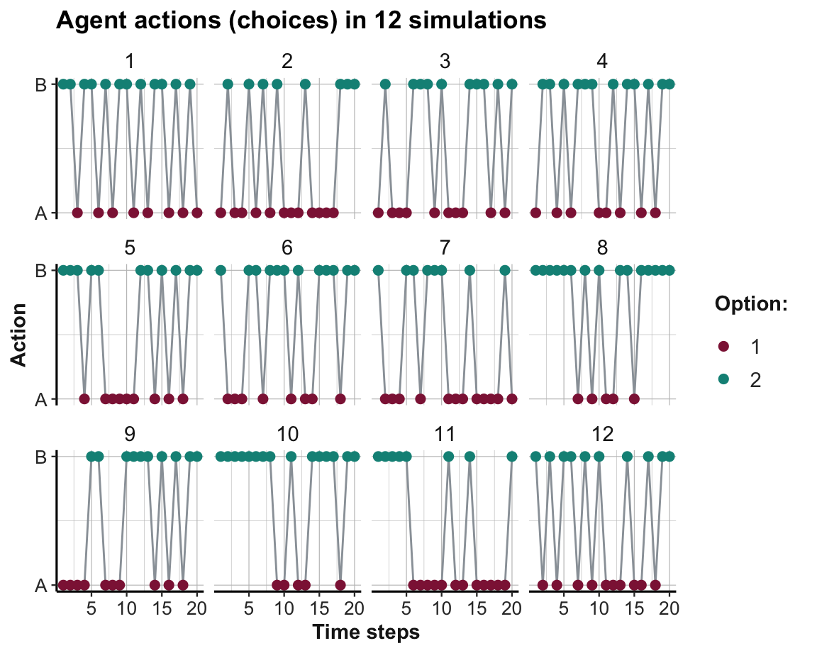

Figure 21.6: The agent’s action (i.e., option chosen) in a binary stochastic MAB per time step and simulation.

As before, Option B still yields higher rewards on average than Option A. However, due to the 50% chance of not receiving a reward for either option, the learning process is made more difficult. Although Figure 21.6 suggests that some agents develop a slight preference for the superior Option B, there are no clear trends within 20 trials. Figure 21.7 shows the option weights per time step for all 12 simulations:

ggplot(data, aes(x = t, group = s)) + 
  geom_path(aes(y = w_A), size = .5, col = usecol(Bordeaux, alpha = .5)) + 
  geom_path(aes(y = w_B), size = .5, col = usecol(Seegruen, alpha = .5)) + 
  labs(title = paste0("Agent weights (expectations/preferences) in ", n_S, " simulations"),   
       x = "Time steps", y = "Weights") + 
  theme_ds4psy()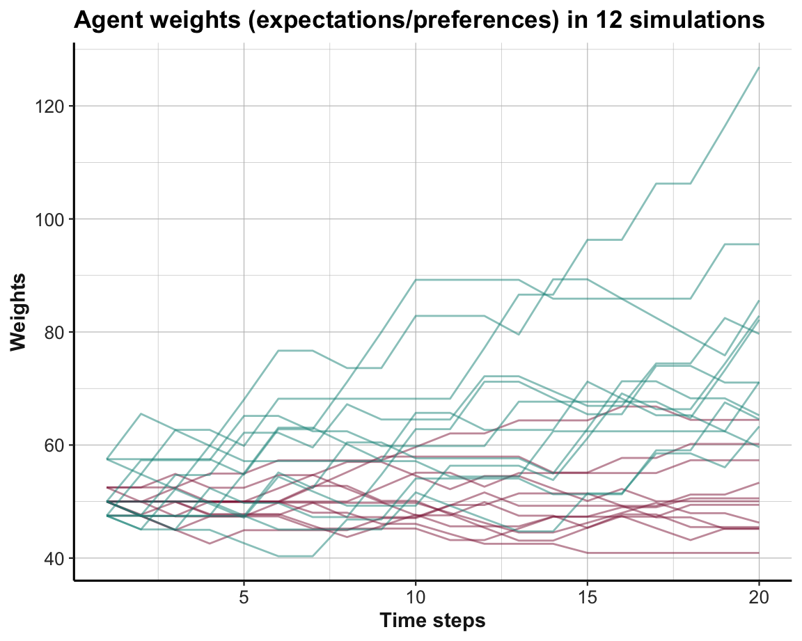

Figure 21.7: Trends in option weights in a binary stochastic MAB per time step for all simulations.

Although there appears some general trend towards preferring the superior Option B (shown in green), the situation is messier than before. Interestingly, we occasionally see that the option weights can also decline (due to negative \(\Delta w\) values, when an option performed below the aspiration level \(A\)).

To document that some systematic learning has occurred even in the stochastic MAB setting, Figure 21.8 shows the average trends in the option weights per time step for all 12 simulations:

ggplot(data, aes(x = t)) + 
  geom_smooth(aes(y = w_A), size = 1, col = usecol(Bordeaux, alpha = .5)) + 
  geom_smooth(aes(y = w_B), size = 1, col = usecol(Seegruen, alpha = .5)) +
  labs(title = paste0("Trends in (average) agent weights in ", n_S, " simulations"),   
       x = "Time steps", y = "Weights", col = "Option:") + 
  theme_ds4psy()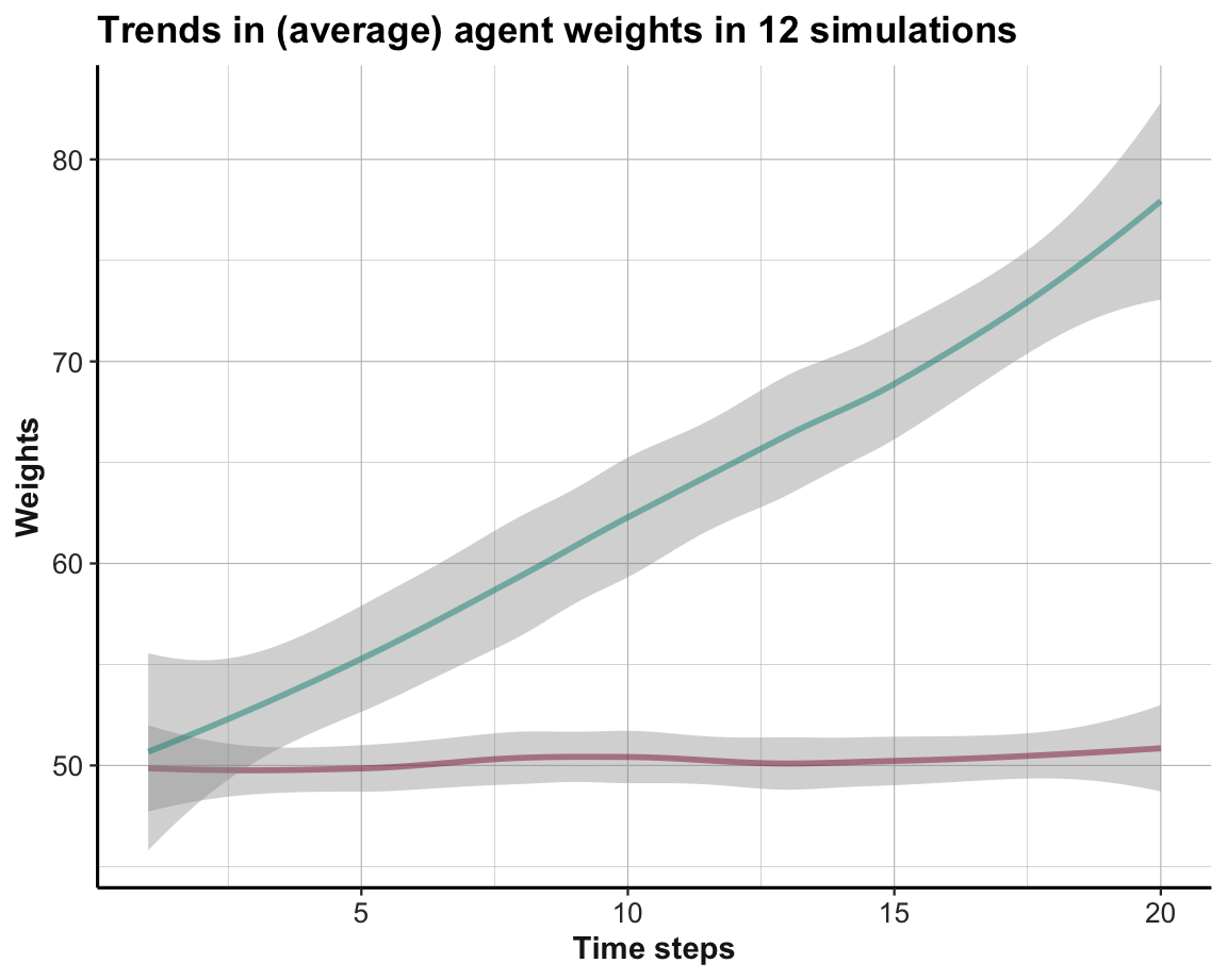

Figure 21.8: Average trends in option weights in a binary stochastic MAB per time step for all simulations.

Interpretation

• The visualization of agent actions (in Figure 21.6) in the MAB setting shows that only a few agents learn to prefer the superior Option B in the n_T = 20 trials.

• The visualization of agent weights (in Figure 21.7) illustrates that agents generally preferred the superior Option B (shown in green) in the second half (i.e., trials 10–20) of the simulation. However, weight values can both increase and decline and the entire situation is much noisier than before, i.e., the preferences are not clearly separated in individual simulations yet.

• However, averaging over the weights for both options (in Figure 21.8) shows that the preference for the better Option B is being learned, even if it does not manifest itself as clearly in the choice behavior yet.

Overall, switching from a stable (deterministic) environment to an uncertain (stochastic) environment rendered the learning task more difficult. But although individual agents may still exhibit some exploratory behavior after n_T = 20 trials, we see some evidence in the agents’ average belief (represented by the average weight values wgt over n_S = 12 agents) that they still learn to prefer the superior Option B over the inferior Option A.

Practice

Answering the following questions improves our understanding of our basic MAB simulation:

1. Describe what the learning agent “expects”, “observes”, and how it reacts, when it initially selects an option, based on whether this option yields its reward value or no reward value.

2. Play with the simulation parameters (n_S and n_T) or agent parameters (alpha) to show more robust evidence for successful learning.

3. How would the simulation results change when the agent’s initial weights (or expectations) were lowered from wgt <- c(50, 50) to wgt <- c(10, 10)? Why?

4. Change the simulation code so that the reward value obtained on every trial is stored as an additional variable in data.

5. Imagine a situation in which a first option yields a lower maximum reward value than a second option (i.e., \(\max \pi(A) < \max \pi(B)\)), but the lower option yields its maximum reward with a higher probability (i.e., \(p(\max \pi(A)) > p(\max \pi(B))\)). This conflict should allow for scenarios in which an agent learns to prefer Option \(A\) over Option \(B\), despite \(B\)’s higher maximum reward. Play with the environmental parameters to construct such scenarios.

Hint: Setting the reward probabilities to rew_prb <- list(c(.8, .2), c(.2, .8)) creates one of many such scenarios. Can we define a general condition that states which option should be preferred?

21.4 Evaluating dynamic models

Models of agents and environments are often created together and hardly distinguishable from each other. Nevertheless, both need to be evaluated. This initially includes ensuring that the agent and environment functions as intended, but also evaluating their performance and the consequences of their interaction. This section illustrates some methods and possible criteria.

21.4.1 Heuristics vs. optimal strategies

Our simulation so far paired a learning agent with a simple MAB problem. However, we can imagine and implement many alternative agent strategies. Typical questions raised in such contexts include:

• What is the performance of Strategy X?

• Is Strategy X better or worse than Strategy Y?

While all MAB settings invite the strategies that balance exploration with exploitation, we can distinguish between two general approaches towards creating and evaluating strategies:

1. Heuristic approaches create and evaluate strategies that are simple enough to be empirically plausible. Heuristics can be defined as adaptive strategies that ignore information to make efficient, accurate and robust decisions under conditions of uncertainty (see Gigerenzer & Gaissmaier, 2011; Neth & Gigerenzer, 2015, for details). As many researchers have a bias to reflexively associate heuristics with inferior performance, we emphasize that simple strategies are not necessarily worse than computationally more expensive strategies. The hallmark of heuristics is that they do not aim for optimality, but rather for simplicity by ignoring some information. Whether they turn out to be worse or better than alternative strategies is an empirical question and mostly depends on the criteria employed.

An example of a heuristic in a MAB setting with stochastic options is sample-then-greedy. This heuristic explores each option for some number \(s\) trials, before exploiting the seemingly better one for the remaining trials. Clearly, the success of this heuristic varies as a function of \(s\): If \(s\) was too small, an agent may not be able to successfully discriminate between options and risk exploiting an inferior option. By contrast, larger values of \(s\) reduce the uncertainty about the options’ estimated rewards, but risk wasting too much trials on exploration.

The same considerations show that the performance of any strategy depends on additional assumptions regarding the nature of the task environment. Estimating the characteristics of an option by sampling it first assumes that options remain stable for the duration of a scenario.

2. Optimality approaches create and evaluate strategies that maximize some performance criterion. Typically, total reward is maximized at the expense of computational effort, but when there is a fixed reward it is also common to minimize the amount of time to reach some goal. There is a lot of scientific literature concerned with the discovery and verification of optimal MAB strategies. Most of these approaches strive for optimization under contraints, which renders the optimization problem even harder.

An example for an optimality approach towards MABs is the computation of the so-called Gittins index for each option. This index essentially incorporates all that can be known so far and computes the value of each option at this moment, given that we only choose optimal actions for all remaining trials (see Page, 2018, p. 322ff., for an example). On every trial, the option with the highest Gittins index is the optimal choice. As this method is conceptually simple but computationally expensive, it is unlikely that organisms solve MAB problems in precisely this way, though they may approximate its performance by other mechanisms.

In a Bayesian agent framework, an agent has prior beliefs about the distribution of rewards of each option and adjusts these beliefs based on its experience in an optimal fashion. Interestingly, however, incorporating experienced rewards in an optimal (or rational) fashion does not yet yield an optimal strategy for choosing actions.

Comparisons between a range of strategies may yield surprising results. For instance, algorithms that perform well on some problems may turn out to be really bad for others. And simple heuristics often outperform theoretically superior algorithms by a substantial margin (Kuleshov & Precup, 2014).

Actually, we typically need a third category to limit the range of possible performances: Baselines.

Need for running competitions between strategies. (See methodology of evaluating models by benchmarking and RTA, below).

21.4.2 Benchmarking strategy performance

Beware of a common fallacy: When evaluating some strategy, researchers often note a deviation between observed performance and some normative model and then jump to premature conclusions (typically by diagnosing the “irrationality” of agents with respect to some task). A typical example of a premature conclusion in the context of a learning task would be to quantify an agent’s total reward \(R_T\) in an environment and contrast it with the maximum possible reward \(R_{max}\) that the environment could have provided. When \(R_T < R_{max}\), a researcher could diagnose “insufficient learning” or “suboptimal performance”. However, this conclusion falls prey to the experimenter’s fallacy of assuming that the agent’s environment corresponds to the experimenter’s environment. In reality, however, the agent views the environment from a different and more limited perspective: Rather than knowing all options and the range of their possible rewards, a learning agent needs to explore and estimate options in a trial-and-error fashion. Thus, an environment that appears to be under risk from the experimenter’s perspective, is typically an uncertain environment from the agent’s perspective. Rather than just making a terminological point, this difference can have substantial consequences for the evaluation of performance — and for implications regarding the agent’s (ir-)rationality (see Sims et al., 2013, for a prominent example).

To vaccinate researchers against drawing premature conclusions regarding the (ir-)rationality of agents, Neth et al. (2016) propose a methodology and perspective called rational task analysis (RTA). RTA is anchored in the notion of bounded rationality (Simon, 1956) and aims for an unbiased interpretation of results and the design of more conclusive experimental paradigms. Rather than the much more ambitious endeavor of rational analysis (Anderson, 1990), RTA focuses on concrete tasks as the primary interface between agents and environments. By providing guidelines for evaluating performance under conditions of bounded rationality, RTA requires explicating essential task elements, specifying rational norms, and bracketing the range of possible performance, before contrasting various benchmarks with actual performance. The recommendations of RTA are summarized in Figure 21.9:

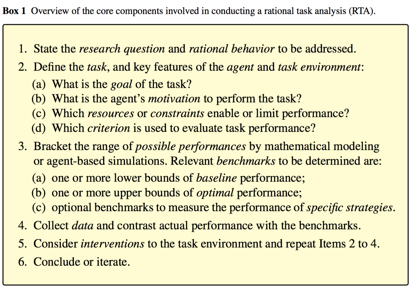
Figure 21.9: The steps of rational task analysis (RTA) according to Neth et al. (2016).

Although the six steps of RTA look like a generic recipe, our evaluations always need to be adapted to the conditions and constraints of specific tasks. However, rather than just comparing some strategy against some normative model, we generally should compare a range of different strategies.

21.5 Conclusion

This chapter made our simulations more dynamic by allowing for incremental changes in agents and environments. This introduced two key topics commonly addressed by computational models: Adaptive agents (i.e., learning) and choice behavior in risky environments (in the form of multi-armed bandits). Additionally, the need for evaluating a variety of strategies raised issues regarding the performance of heuristics relative to baseline and optimal performance.

21.5.1 Summary

Most dynamic simulations distinguish between some agent and some environment and involve step-wise changes of internal states, environmental parameters, or their interactions (e.g., typically described as behavior). We distinguished between various locations and types of changes:

1. The phenomenon of learning involved changing agents that adapt their internal states (e.g., beliefs, preferences, and actions) to an environment.

2. The MAB paradigm allowed for changes in environments whose properties are initially unknown (with risky or uncertain options)

3. The interaction between agents and environments raised questions regarding the performance of specific strategies (e.g., models of different learning mechanisms and heuristics). Performance should always be evaulated relative to sound benchmarks (ideally of both baseline and optimal performance).

Learning agents that interact with dynamic, risky and uncertain environments are a key topic in the emerging fields of artificial intelligence (AI) and machine learning (ML). Although we only took a peek at the surface of these models, we can note some regularities in the representations used for modeling the interactions between agents and environments:

• time is represented as steps: The states of agents and environments can change

• agent beliefs and representations of their environments as probability distributions

• environments as a range of options (yielding rewards or utility values), that can be stable, risky, or uncertain, deterministic or probabilistic

This is progress, but still subject to many limitations. Two main constraints so far were that the nature or number of options did not change and that we only considered an individual agent.

Additional sources of variability

Adding uncertainty to payoff distributions is only a small step towards more dynamic and realistic environments. We can identify several sources of additional variability (i.e., both ignorance and uncertainy):

1. Reactive and restless bandits:
   How do environments respond to and interact with agents? Many environments deplete as they are exploited (e.g., patches of food, fish in the sea, etc.), but some also grow or improve (e.g., acquiring expertise, playing an instrument, practicing some sport).
   Beyond providing rewards based on a stable probability distribution, environments may alter the number of options (i.e., additional or disappearing options), the reward types or magnitudes associated with options, or the distributions with which options provide rewards. All these changes can occur continuously (e.g., based on some internal mechanism) or suddenly (e.g., by some disruption).

2. Multiple agents:
   Allowing for multiple agents in an environment changes an individual’s game against nature by adding a social game (see the chapter on Social situations). Although this adds many new opportunities for interaction (e.g., social influence and social learning) and even blurs the conceptual distinction between agents and environments, it is not immediately clear whether adding potential layers of complexity necessarily requires more complex agents or simulation models (see Section 22.1.1).

Some directions for possible extensions include:

• More dynamic and responsive environments (restless bandits):

  • MAB with a fixed set of options that are changing (e.g., depleting or improving)

  • Environments with additional or disappearing options

• Social settings: Multiple agents in the same environment (e.g., games, social learning).

Note that even more complex versions of dynamic simulations typically assume well-defined agents, environments, and interactions. This changes when AI systems are moved from small and closed worlds (e.g., with a limited number of risky options) into larger and more open worlds (e.g., with a variable number of options and uncertain payoffs). Overall, modeling a video game or self-driving car is quite a bit more challenging than a multi-armed bandit.

Fortunately, we may not always require models of optimal behavior for solving problems in real-world environements. Simon (1956) argues that an agent’s ability to satisfice (i.e., meeting some aspiration level) allows for simpler strategies that side-step most of the complexity faced when striving for optimal solutions.

Another important insight by Herbert Simon serves as a caveat that becomes even more important when moving from small worlds with fixed and stable options into larger and uncertain worlds:

An ant, viewed as a behaving system, is quite simple.
The apparent complexity of its behavior over time is largely a reflection
of the complexity of the environment in which it finds itself.

(Simon, 1996, p. 52)

Essentially, the complex challenges posed by real-world problems do not necessarily call for complex explanations, but they require that we are modeling the right entity. Whereas researchers in the behavioral and social sciences primarily aim to describe, predict, and understand the development and behavior of organisms, they should also study the structure of the environments in which behavior unfolds. Thus, successful models of organisms will always require valid models of environments.

21.5.2 Resources

This chapter only introduced the general principles of learning and multi-armed bandit (MAB) simulations. Here are some pointers to sources of much more comprehensive and detailed treatments:

Reinforcement learning

• The classic reference to RL is the book by Sutton and Barto (originally published in 1992). Its second edition (Sutton & Barto, 2018) is available at http://incompleteideas.net/book/the-book-2nd.html.

• A more concise, but mathematical overview of RL is provided by Szepesvári (2010), which is available at https://sites.ualberta.ca/~szepesva/rlbook.html.

• Silver et al. (2021) argue that the goal of maximising reward may be the key to understanding the intelligence of natural and artificial minds.

• Some excellent courses on RL are available at https://deepmind.com/learning-resources. For instance, this 10-session introduction to RL by David Silver.

Multi-armed bandits (MABs)

• The article by Kuleshov & Precup (2014) provides a comparison of essential MAB algorithms and shows that simple heuristics can outperform more elaborate strategies. It also applies the MAB framework to the allocation of clinical trials.

• The book by Lattimore & Szepesvári (2020) provides abundant information about bandits and is available here. The blog Bandit Algorithms provides related information in smaller units.

21.6 Exercises

Here are some exercises for simple learning agents that interact with stable or dynamic environments.

21.6.1 Learning with short-term aspirations

Our basic learning model (developed in Section 21.2) assumed that a learning agent has a constant aspiration level of \(A = 5\). As the reward from selecting the worst option still exceeds \(A\), this always leads to a positive “surprise” upon receiving a reward, corresponding increments of \(\Delta w > 0\), and monotonic increases in weight values wgt. Although having low expectations may guarantee a happy agent, it seems implausible that an agent never adjusts its aspiration level \(A\). This exercise tries the opposite approach, by assuming an extremely myopic agent who always updates \(A\) to the most recent reward value:

1. Adjust \(A\) to the current reward value on each trial \(t\).

Hint: This also requires that the current reward value is explicitly represented in each loop, rather than only being computed implicitly when calling the delta_w() function.

2. Does the agent still successfully learn to choose the better option? Describe how the learning process changes (in terms of the values of \(A\) and \(wgt\), and the options being chosen).

3. Given the new updating mechanism for \(A\) and assuming no changes in the agent’s learning rate alpha, the initial wgt values and delta_w(), how could a change in the probability of choosing options (i.e., the p() function) increase the speed of learning?

4. Explain why it is essential that \(A\) is adjusted after updating the agent’s wgt values. What would happen, if an agent prematurely updated its aspiration level to the current reward (prior to updating wgt)?

Solution

• ad 1.: We copy the functions p(), r() and delta_w(), as defined in Section 21.2:

# 1. Choosing: 
p <- function(k){  # Probability of k:
  
  wgt[k]/sum(wgt)  # wgt denotes current weights
  
}

# Reward from choosing k: 
r <- function(k){
  
  rew[k]  # rew denotes current rewards
  
}

# 2. Learning: 
delta_w <- function(k){  # Adjusting the weight of k: 
  
  (alpha * p(k) * (r(k) - A))
  
}

the following code extends the code from above in two ways:

• After updating wgt, the current reward value cur_rew is explicitly determined (for a second time) and the aspiration level A is set to this value on each individual trial (see Step 3 within the inner loop);

• data is extended to include the current value of A (or cur_rew) on each individual trial.

# Simulation:
n_S <- 12  # number of simulations     
n_T <- 20  # time steps/cycles (per simulation)

# Environmental constants: 
alt <- c("A", "B")  # constant options
rew <- c(10, 20)    # constant rewards (A < B)

# Prepare data structure for storing results: 
data <- as.data.frame(matrix(ncol = (4 + length(alt)), nrow = n_S * n_T))
names(data) <- c("s", "t", "act", "A", paste0("w_", alt))

for (s in 1:n_S){     # each simulation: ---- 
  
  # Initialize agent: 
  alpha <- 1        # learning rate
  A <- 5            # aspiration level
  wgt <- c(50, 50)  # initial weights 
  
  for (t in 1:n_T){   # each step/trial: ---- 
    
    # (1) Use wgt to determine current action: 
    cur_prob <- c(p(1), p(2))
    cur_act <- sample(alt, size = 1, prob = cur_prob)
    ix_act <- which(cur_act == alt)

    # (2) Update wgt (based on reward): 
    new_w <- wgt[ix_act] + delta_w(ix_act)  # increment weight
    wgt[ix_act] <- new_w  # update wgt
    
    # (3) Determine reward and adjust A:
    cur_rew <- rew[ix_act]  # value of current reward
    A <- cur_rew            # update A
    
    # (+) Record results:
    data[((s-1) * n_T) + t, ] <- c(s, t, A, ix_act, wgt)
    
  } # for t:n_T end.
  
  print(paste0("s = ", s, ": Ran ", n_T, " steps, wgt = ", 
               paste(round(wgt, 0), collapse = ":"), 
               ", A = ", A))
  
} # for i:n_S end.
#> [1] "s = 1: Ran 20 steps, wgt = 34:76, A = 10"
#> [1] "s = 2: Ran 20 steps, wgt = 33:79, A = 10"
#> [1] "s = 3: Ran 20 steps, wgt = 43:66, A = 20"
#> [1] "s = 4: Ran 20 steps, wgt = 33:86, A = 20"
#> [1] "s = 5: Ran 20 steps, wgt = 37:76, A = 20"
#> [1] "s = 6: Ran 20 steps, wgt = 31:83, A = 10"
#> [1] "s = 7: Ran 20 steps, wgt = 39:72, A = 20"
#> [1] "s = 8: Ran 20 steps, wgt = 43:66, A = 20"
#> [1] "s = 9: Ran 20 steps, wgt = 30:94, A = 20"
#> [1] "s = 10: Ran 20 steps, wgt = 33:79, A = 10"
#> [1] "s = 11: Ran 20 steps, wgt = 30:94, A = 20"
#> [1] "s = 12: Ran 20 steps, wgt = 29:97, A = 20"

# Report result:
print(paste0("Finished running ", n_S, " simulations (see 'data' for results)"))
#> [1] "Finished running 12 simulations (see 'data' for results)"

The printed summary information after each simulation shows that all agents seem to successfully discriminate between options (by learning a higher weight for the superior Option B).

• ad 2.: From the 2nd trial onwards, the agent always aspires to its most recent reward. Thus, the agent is never surprised when the same reward is chosen again and only learns upon switching options:

  • When switching from Option A to Option B, the reward received exceeds \(A\), leading to an increase in the weight for Option B.

  • When switching from Option B to Option A, the reward received is lower than \(A\), leading to an decrease in the weight for Option A. This explains why the weights of Option A can decrease and generally are lower than their initial values in this simulation.

• ad 3.: Given this setup, the pace of learning depends on the frequency of switching options. Increasing the agent’s propensity for switching would increase its learning speed.

• ad 4.: If Steps 2 and 3 were reversed (i.e., A was updated to the current reward value prior to updating wgt), the difference r(k) - A in delta_w() would always be zero. Thus, the product \(\Delta w(k)\) will always be zero, irrespective of \(k\) or \(t\). Overall, the premature agent would never learn anything. (Consider trying this to verify it.)

21.6.2 Learning with additional options

This exercise extends our basic learning model (from Section 21.2) to a stable environment with additional options:

1. Extend our learning model to an environment with three options (named A, B, and C) that yield stable rewards (of 10, 30, and 20 units, respectively).

2. Visualize both the agent choices (i.e., actions) and expectations (i.e., weights) and interpret what they show.

3. Assuming that the options and rewards remain unchanged, what could improve the learning success? (Make a prediction and then test it by running the simulation.)

Solution

• ad 1.: Still using the functions p(), r() and delta_w(), as defined in Section 21.2:

# 1. Choosing: 
p <- function(k){  # Probability of k:
  
  wgt[k]/sum(wgt)  # wgt denotes current weights
  
}

# Reward from choosing k: 
r <- function(k){
  
  rew[k]  # rew denotes current rewards
  
}

# 2. Learning: 
delta_w <- function(k){  # Adjusting the weight of k: 
  
  (alpha * p(k) * (r(k) - A))
  
}

the following code extends the simulation from above to three options:

# Simulation:
n_S <- 12  # number of simulations     
n_T <- 20  # time steps/cycles (per simulation)

# Environmental constants: 
alt <- c("A", "B", "C")  # constant options
rew <- c(10, 30, 20)     # constant rewards

# Prepare data structure for storing results: 
data <- as.data.frame(matrix(ncol = (3 + length(alt)), nrow = n_S * n_T))
names(data) <- c("s", "t", "act", paste0("w_", alt))

for (s in 1:n_S){  # each simulation: ---- 
  
  # Initialize learner: 
  wgt <- c(50, 50, 50)  # initial weights 
  alpha <- 1  # learning rate
  A <- 5      # aspiration level
  
  for (t in 1:n_T){  # each step: ---- 
    
    # (1) Use wgt to determine current action: 
    cur_prob <- c(p(1), p(2), p(3))
    cur_act <- sample(alt, size = 1, prob = cur_prob)
    ix_act <- which(cur_act == alt)
    
    # (2) Update wgt (based on reward):
    new_w <- wgt[ix_act] + delta_w(ix_act)  # increment weight
    wgt[ix_act] <- new_w  # update wgt
    
    # (+) Record results:
    data[((s-1) * n_T) + t, ] <- c(s, t, ix_act, wgt)
    
  } # for t:n_T end.
  
  print(paste0("s = ", s, ": Ran ", n_T, " steps, wgt = ", 
               paste(round(wgt, 0), collapse = ":")))
  
} # for i:n_S end.
#> [1] "s = 1: Ran 20 steps, wgt = 55:157:78"
#> [1] "s = 2: Ran 20 steps, wgt = 53:196:67"
#> [1] "s = 3: Ran 20 steps, wgt = 56:146:77"
#> [1] "s = 4: Ran 20 steps, wgt = 53:110:108"
#> [1] "s = 5: Ran 20 steps, wgt = 63:149:56"
#> [1] "s = 6: Ran 20 steps, wgt = 56:144:78"
#> [1] "s = 7: Ran 20 steps, wgt = 59:116:84"
#> [1] "s = 8: Ran 20 steps, wgt = 57:71:124"
#> [1] "s = 9: Ran 20 steps, wgt = 61:117:77"
#> [1] "s = 10: Ran 20 steps, wgt = 61:70:110"
#> [1] "s = 11: Ran 20 steps, wgt = 60:125:76"
#> [1] "s = 12: Ran 20 steps, wgt = 58:157:68"

• ad 2.: As before, the data frame data collects information on all intermediate states. This allows us to visualize the learning process in terms of the actions chosen (choices):

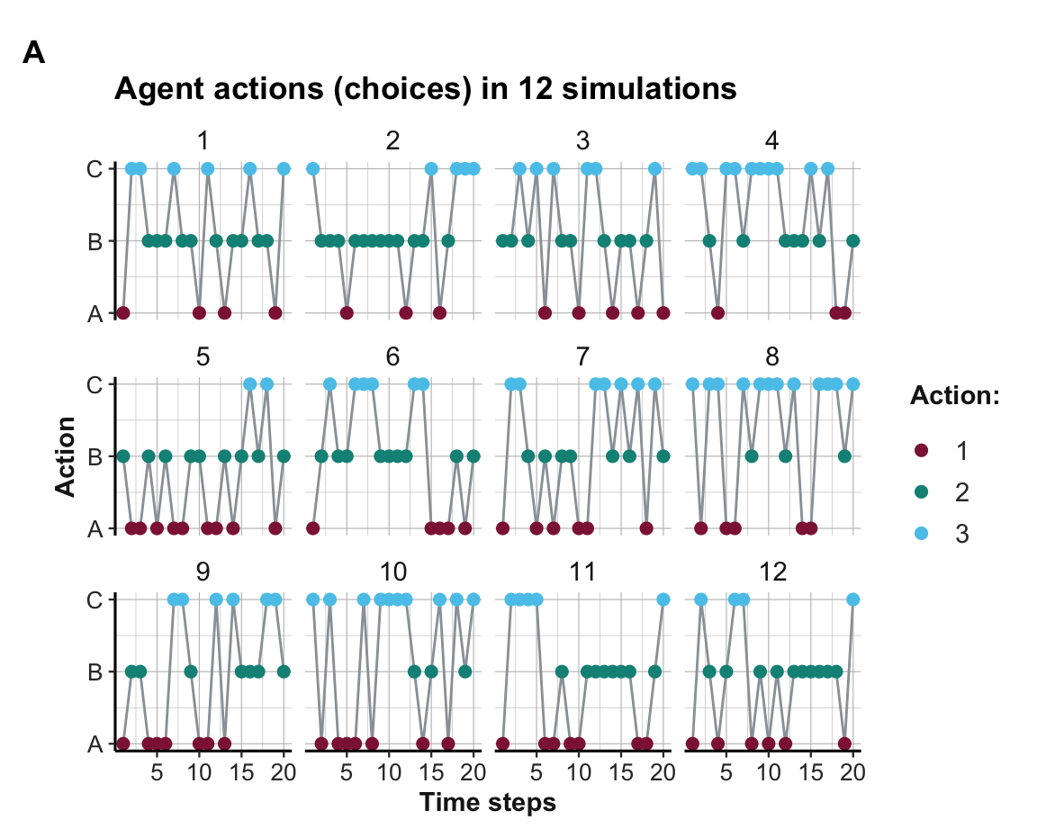
Figure 21.10: Options chosen (over 12 simulations).

internal expectations (weight values):

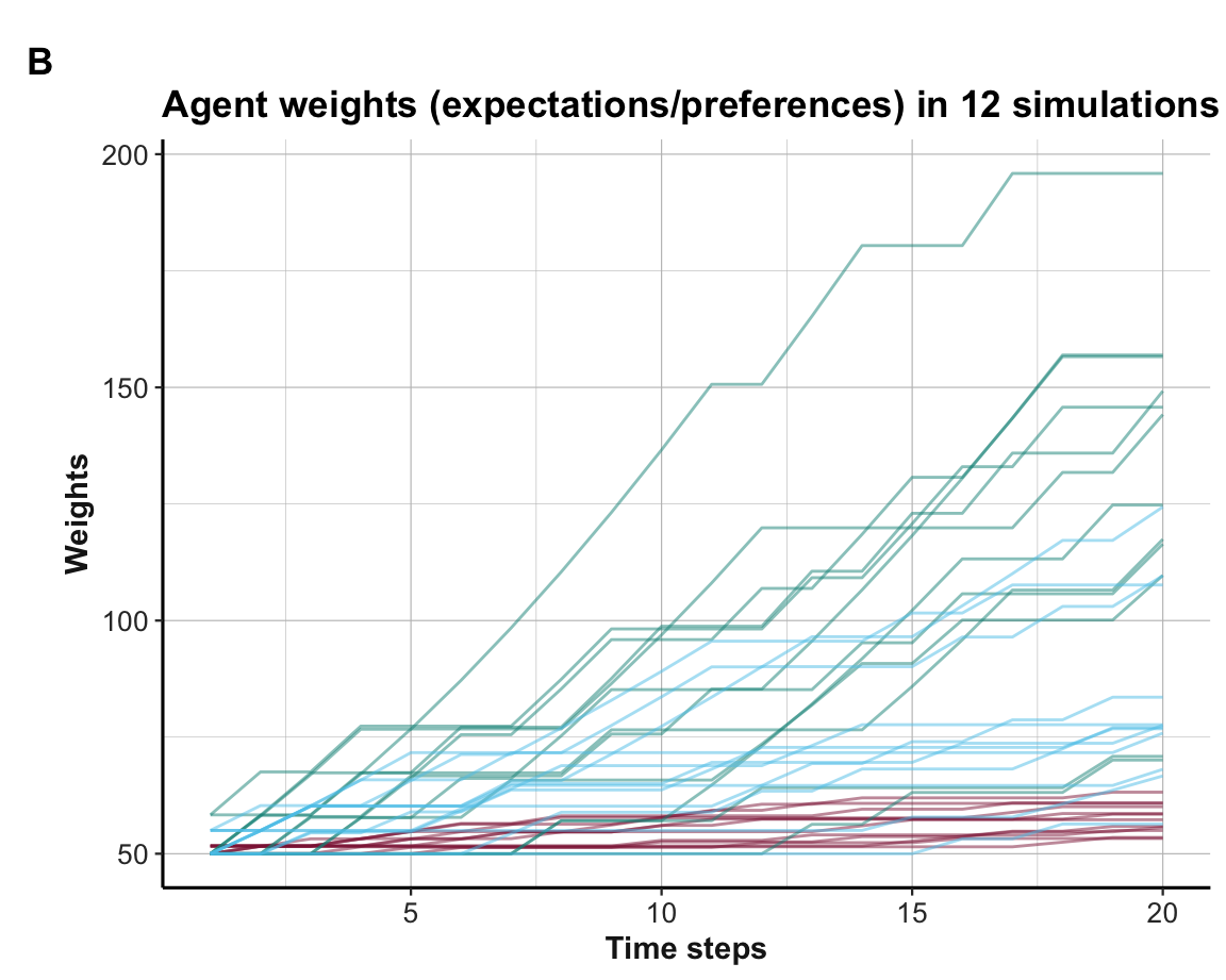
Figure 21.11: Weight values (over 12 simulations).

and their average trends:

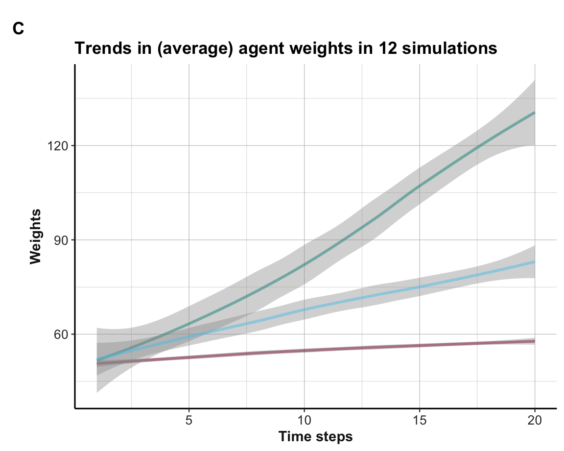
Figure 21.12: Average trends in weight values.

Interpretation

The plot of agent actions (A) shows that some, but not all agents learn to choose the best Option B within 20 rounds. Due to the more complicated setup of three options and their more similar rewards, the learning is slower and not always successful. This is also reflected in the visualization of the weights (shown in B), which are not separated as cleanly as in the binary case (see Section 21.2). However, the average trends (shown in C) still provide systematic evidence for learning when averaging the agent weight values over all 12 simulations.

• ad 3.: Increasing the learning rate (e.g., to \(\alpha = 2\)) or increasing the number of trials \(n_T\) per simulation both lead to better (i.e., faster or more discriminating) learning.

21.6.3 A foraging MAB

Create a model of a multi-armed bandit as a dynamic simulation of a foraging situation:

• Environment with 3 options, with dynamic rewards (either depleting or improving with use).

• Assess the baseline (e.g., random) and the optimal performance (when knowing the definition of the environment).

• Assess the performance of 2 learning agents (with different parameters) and 2 heuristics (without learning).

21.6.4 Maximization vs. melioration

A deep puzzle regarding the adaptive behavior of organisms concerns the mechanism that leads to adaptation and learning. In principle, two alternative mechanisms are possible:

• maximizing: Selecting the best option (global optimization)
• meliorating: Selecting the better option (local optimization)

In most environments, both mechanisms will be correlated and converge on the same option(s). However, consider the following environment:

• There are two buttons/options for max (for maximizing) or mel (for meliorating).

• The reward or value of each option depends on the current system state x. The value of x is defined as a function of the past \(w=10\) choices. Specifically, x is defined as the proportion of max choices over the \(w=10\) most recent choices.

• The value of choosing max or mel for any value of x is shown in Figure 21.13
  (on the y-axis, which may denote the magnitude of a reward or the probability of receiving a constant reward).

Figure 21.13: A dynamic 2-armed bandit that contrasts maximization with melioration.

• The rewards for meliorating (curve mel(x), in red) are always higher than the rewards for maximizing (curve max(x), shown in green). As both lines are parallel, the difference is always given by \(B\), regardless of the value of x.

Your tasks

1. Implement this environment as a simulation in R.

2. Implement some simple strategies (e.g., a random strategy, a win-stay/lose-shift strategy, etc.) and evaluate their performance. Which strategies are most successful?

3. Try implementing a learning strategy. What does the strategy learn?

Note

Environments of this type have extensively been studied by Richard Herrnstein and colleagues (Herrnstein, 1991; Herrnstein & Prelec, 1991; e.g., Herrnstein & Vaughan, 1980; Rachlin & Laibson, 1997). The implications of these experiments have been examined in Sims et al. (2013).

---

32. Page (2018) uses the Greek letter \(\gamma\) as the learning rate. But as some learning models also use \(\gamma\) as a discount factor that determines the importance of future rewards, we denote the learning rate by the more common letter \(\alpha\) here.↩︎

33. As r() is called by delta_w(), this creates a functional dependency in our model that renders some information implicit (here: the value of the reward received on every trial). As we will see, models often need to balance concerns for elegance and practicality.↩︎

34. We use a reduced learning rule (which replaces \(p(k)\) by a constant of 1) to obtain the same values as in Page (2018) (p. 308).↩︎