11 Importing data
Where does data come from? In the vast majority of cases, the data we analyze was not generated by ourselves. Instead, we find or are provided with data that is of interest to us. As such data may stem from a variety of sources, it is usually not pre-processed or stored in R. Thus, a non-trivial question that needs to be answered is:
- How can we get our data into R?
In R, we generally get data — typically as vectors or tables — by importing it from some file or by creating it from scratch. In both cases, we usually want to end up with a rectangular data structure known as a “tibble”, which is a simplified version of an R data frame.
The two key topics of this and the next chapter (Chapter 12) are:
Reading and writing data files with the readr package (Wickham, Hester, et al., 2024)
Creating tibbles with the tibble package (Müller & Wickham, 2023)
Both these packages belong to the so-called tidyverse (Wickham et al., 2019) and create a rectangular data structure known as a “tibble”. While these packages are more consistent than the corresponding base R functions, the utils package also contains generic functions for reading and writing files. While tibbles tend to be more convenient than data frames, we can usually get by just fine by using standard data frames, rather than tibbles.
An important precondition for working productively with R (or any other programming language) is that we have some basic understanding of file systems and storage locations. Thus, this chapter needs to briefly explain the notion of (absolute or relative) paths and how to organize R projects.
Preparation
Recommended readings for this chapter include
- Chapter 7: Data import of the 2nd edition of r4ds (Wickham, Çetinkaya-Rundel, et al., 2023)
- Chapter 6: Importing data of the ds4psy book (Neth, 2023a).
For a more comprehensive overview of using R projects and readr, see the corresponding chapters of the r4ds book (Wickham & Grolemund, 2017):
Preflections
Before reading, please take some time to reflect upon the following questions:

If we were interested in answering some interesting question, what data would we require?
Where do we get data from?
If someone had all the data we need, how would we obtain, load or enter it into R?
How can we load a data file from another directory or a different machine?
How would we store or share our data?
In this chapter, we will learn how to orient ourselves on our computer, and how to create, read, and write tabular data structures in R.
11.1 Introduction
Data is rarely entered directly into R. When we analyze data, getting data into R can either imply
importing data from some file or server (see Section 11.3), or
creating data from other R data structures or from scratch (see Chapter 12).
In both cases, we aim to end up with rectangular data structure known as a “tibble”, which is a simplified type of data frame, used in the tidyverse (Wickham et al., 2019). But tibbles are not just an end result of getting and analyzing data — we may also want to share them with others. This requires saving (or “writing”) our data to files into some folder in a form that allows us or others to re-load them (into R or other programs).
Figure 11.1 provides an initial overview of the roles of the readr and tibble packages: Both packages help to create tibbles, but differ in their input sources. Existing tibbles can then be used for data analysis in R (e.g., for data transformations, visualizations, or statistics) or can be written to files (e.g., to be archived locally or shared online).
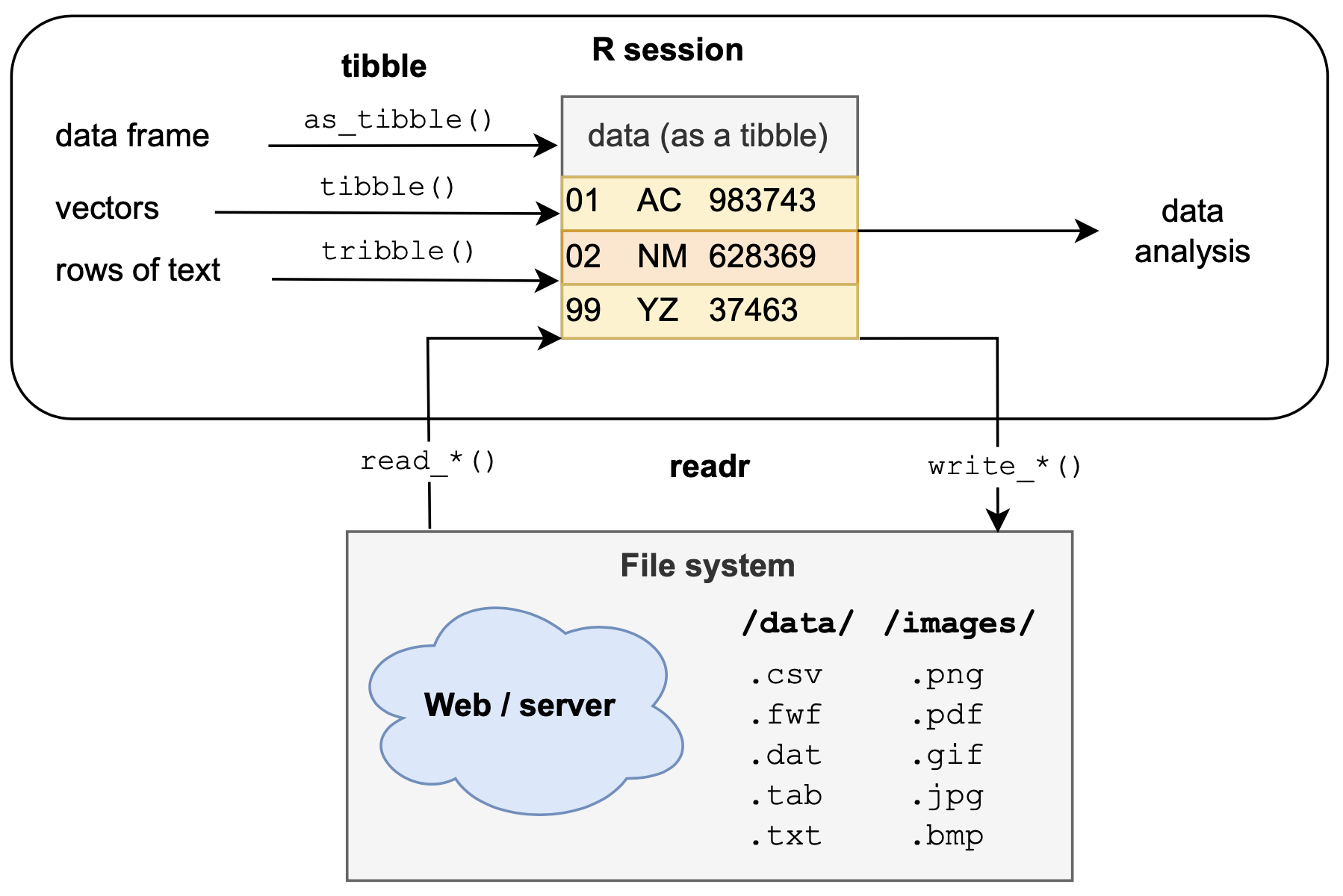
Figure 11.1: The readr and tibble packages use different inputs to create a tabular data structure known as a tibble, which is a simpler data frame. Tibbles can be then used for data analysis in R (e.g., for transforming or visualizing data, or statistical testing) or written to a file (e.g., for archival or sharing purposes).
A typical R workflow includes not only reading and writing files, but also that we are oriented in our current computing environment. This implies that we can navigate between folders, can describe and link to files, and know how to organize an R project (see Section 11.2).
Terminology
Key concepts of Section 11.2 on getting oriented and organized include:
- files and folders
- R’s working directory
- paths (absolute vs. relative)
- R projects
Key concepts of Section 11.3 on importing data include:
- parsing (vectors or files)
- importing/reading vs. exporting/writing files
Resources
The resources used in this chapter on importing data include:
functions from the base R package utils and the tidyverse package readr (Wickham, Hester, et al., 2024)
data from the ds4psy package (Neth, 2023b) and the palmerpenguins package (Horst et al., 2022)
Some text sections will link to corresponding sections of Chapter 6: Importing data of the ds4psy book (Neth, 2023a).
To practice importing external files of various formats, some data files are stored at rpository.com.
Before we can begin importing data into R, we need to get oriented on our computers.
11.2 Getting oriented and organized
Modern computer systems usually provide some sort of graphical user interface, that visualizes the contents of our hard drives as files that are stored in directories (or folders). Given fancy interactive devices (like a mouse or a track pad), the task of navigating between folders and moving files becomes a perceptual-motor task that involves clicks and gestures. Although this may be more convenient than typing into a terminal, some knowledge of location descriptions (or “paths”) is helpful when working with R (or any other programming language).
Our R system operates within an infrastructure that consists of many files and folders, but also other programs and computers. When adopting the perspective of our R system, we can always ask:
- Where am I?
- Where is the data?
The answer to the first question is known as R’s current working directory.
R’s working directory
Any R session is running in its current working directory.
As we can start R from various locations (e.g., locally or on a remote server), the working directory is not necessarily the same directory as the location of an R file that we are editing or evaluating.
A well-organized project typically contains various (sub-)directories for storing different types of data.
For instance, larger projects contain dedicated sub-directories for data, images, or R code files.
To determine the current working directory, we can use the getwd() function of base R.
For the i2ds book, the working directory is:
getwd()
#> [1] "/Users/hneth/Desktop/stuff/Dropbox/GitHub/i2ds_book"
Note that evaluating the getwd() function returns a directory path, which is the description of a location on a computer (as a character string). This path depends both on our operating system (e.g., its hierarchy of directories) and on the specific organization of our local file system.
If we wanted to change R’s working directory, we could use the setwd() function and provide an alternative location in its dir argument. For instance, the following code would first save R’s current working directory (as wd) and then change it to another directory, before changing it back to the original directory:
# 0. store original working directory:
wd <- getwd()

# 1. Change to a different working directory:
setwd(dir = "/Users/hneth/Desktop/stuff/")
getwd()  # verify new working directory
#> [1] "/Users/hneth/Desktop/stuff"

# 2. Re-set original working directory:
setwd(wd)
Given such functions to find out and change our working directory, we can ask:
- Why would we want to know or change our working directory?
The fact that we often work with multiple projects and not all files are stored in the same directory make it necessary to know or set one’s current working directory, as well as point to the locations of files in other directories. When working with projects in the RStudio IDE, R sets a session’s original working directory to the project folder.
To get and stay oriented on our computers, we need to disentangle two aspects: The location at which some object of interest (e.g., a data or image file) is being stored vs. how we refer to this location (i.e., its path). Whereas the storage location of objects can be local or remote, their paths can be expressed in absolute or relative ways. While the distinction between “local” and “remote” objects is always relative to the current working directory, any particular object can be described by both its absolute or its relative path.
11.2.1 Local vs. remote locations
The reason to know and possibly change our working directory is that we frequently need to access (e.g., read or write) files that are located elsewhere (i.e., in other directories). The notion of “elsewhere” is deliberately vague: If we only consider files within our working directory as “local”, all other files are “remote”. Thus, a remote file A can be located in a sub-directory of our working directory and a remote file B on an online server at the other end of the world. From R’s perspective, both files are remote by not being located in the working directory.
The list.files() function shows us the local files of a directory.
For instance, to see the files and directories of our working directory, we could evaluate:
list.files() # list local files and directoriesWhen aiming to access a remote file, we could change our working directory to this other location, so that the file becomes local. However, the more common way of dealing with such situations is to retain our current working directory and describe the location of the remote file by its path.
11.2.2 Absolute vs. relative paths
The second question from above (“Where is the data?”) can be answered in two ways, but both involve specifying a path to the data. File paths are not locations, but rather descriptions of locations on a computer, typically expressed as character strings. Whenever aiming to read or write files that are not stored in our current working directory, we need to specify their path. Similarly, linking between files or to media contents (e.g., an image) requires providing their file paths.
We can distinguish between two types of file paths:
absolute paths are a top-down description of locations (or the “address” of a file or directory) on a computer. Unfortunately, the way in which file paths are expressed can vary between computer operating systems (but we can always evaluate
getwd()in R to see how our own computer expresses absolute paths). Absolute paths always include the root directory of a particular machine. On UNIX-like systems, the root directory is denoted by/(i.e., a forward slash). When accessing a file from an online server, its absolute path may include elements of URL addresses (likehttpsorwww).relative paths are descriptions of locations (or the “address” of a file or directory) relative to the current working directory. For instance, if my current working directory was
/Users/hneth/project_1, then"/data/my_data.tab"(as a character string) provides a relative path to a filemy_data.tabthat is located in adatasub-directory of theproject_1directory. Thus, the absolute path of this file is/Users/hneth/project_1/data/my_data.tab.
When specifying file paths, some abbreviations are helpful. The most common ones are:
.(i.e., the dot symbol) denotes the current location (i.e., working directory)..(i.e., two dot symbols) denote the current parent directory (i.e., “one level up in the hierarchy”)~(i.e., the squiggly tilde symbol) denotes a user’s home directory
As . and .. are always interpreted relative to the current location, they are used when specifying relative (or local) paths. By contrast, ~ is an abbreviation for an absolute (or global) path.
Importantly, absolute and relative paths can point to the same locations — they really are just two different ways of pointing to an address (typically directories or files on our computer). But as local paths are always interpreted relative to the current working directory, the same local path points to different locations when we begin in a different working directory.
Thinking of two different locations on a map may help: To find out how to get from our current location \(A\) to another location \(B\), we can either look up the absolute/global address of \(B\) (i.e., using street names, numbers, or the map’s coordinate system) or provide directions in a relative/local fashion by adopting \(A\)’s perspective (i.e., “keep going, turn right on the 2nd street, then straight ahead, before turning left at…”). Whereas the absolute address of \(B\) is independent of our current location \(A\), providing relative directions (e.g., “turn right”) assumes knowledge of and always depends on our current location \(A\). Thus, although the absolute and relative descriptions differ, they can both point from \(A\) to \(B\), or retrieve something from \(B\) that is needed at \(A\).
If both types of file paths can describe the same location, why does their difference matter for us? Importantly, global paths always contain the top-level directories of a particular computer, whereas local paths can ignore those machine-specific details. As long as all files that belong together are transferred together with their directory structure, local paths are preferable (and work in the same way as local directions do, provided that the relation between the initial and final locations is preserved). By contrast, global file paths differ between different computers and should therefore be avoided in our code (or must be clearly marked as being user- or machine-specific, if they are being used).
11.2.3 Organizing R projects
As R projects typically consist of multiple files and folders, we need to care about file paths when we ever want to share code or transfer projects to a different machine. The following strategy is based on design principles of websites, which face and solve the same problem:
Anchor every project in a home directory and identify this directory by its absolute path.
Store all files belonging to the project in sub-directories of the home directory, and identify these files by using their relative paths (e.g., express all links to data or image files relative to the home directory).
When accessing to external files (i.e., files not stored within the home directory), refer to these files by their absolute paths (and identify them prominently, e.g., at the top of your main project file).
Following these guidelines makes an R project as self-contained and transferable as possible.
Similar strategies are adopted for designing R packages
(for details, see the Section on Package subdirectories in the manual on Writing R extensions) or when we use the
RStudio IDE for defining a “project”.
The key advantage of these principles is that we can transfer an entire project from one location to another (on the same or a different machine).
Once we re-set the project’s home directory (e.g., by calling getwd() or by using the here() function of the here package), everything else continues to work (provided that we transferred the entire content of the home directory and only used local paths to identify files in its sub-folders).
Defining remote paths
If our project needs to access files from external projects or locations that cannot be easily stored within our project (e.g., data files that are too large to copy or images that are being hosted on external servers), it is useful to store their paths as R objects that provide their absolute paths. For instance, the source code of this book defines R objects for the current URLs of the i2ds and ds4psy textbooks (as character strings):
url_i2ds_book   <- "https://bookdown.org/hneth/i2ds/"
url_ds4psy_book <- "https://bookdown.org/hneth/ds4psy/"
The advantage of specifying external URLs as R objects within our project is that we only need to change the object definition once, if the online address of our project changes (which is quite common for web addresses).
Showing a local image (using its relative path)
As both these directories contain sub-directories for data and images, we can link to their files by specifying either their local or their global paths.
When working within our i2ds project, it is preferable to define a relative file path to link to its cover image:
# Relative path to an image (in a local sub-directory):
my_image <- "./images/cover.png"  # use local path
Provided that my_image denotes a valid path (i.e., there is an image at this location), we can include it in our R Markdown file as follows:
# Include an image (using its relative path):
knitr::include_graphics(path = my_image)
Figure 11.2: A local image identified by its relative path.
Incidentally, the expression knitr::include_graphics() is a way to call the include_graphics() function of the knitr package. Thus, expressions like pkg::fun() are yet another way to denote paths in R (in this case, the call is interpreted relative to our current library of R packages).
Showing an online image (using its absolute path)
However, when aiming to show an image from a different project (e.g., from the ds4psy textbook), it is better to specify and use its global path (even if we had access to the file on our local computer). Assuming that we know an location online of the image, we could do this by specifying its absolute path as an R object:
# Absolute path to an image (available online):
my_image <- "https://bookdown.org/hneth/ds4psy/images/cover.png"

# As URL and (remote) sub-directory:
my_image <- paste0(url_ds4psy_book, "images/cover.png")
As file paths are of data type “character” (i.e., strings of text), we can use text manipulation functions like paste0() to construct the desired path from its parts (e.g., the URL defined above and a remote sub-directory).
Again, provided that my_image denotes a valid path (i.e., there is an image at this location), we can include it in our R Markdown file as before:
# Include an image (using its absolute path):
knitr::include_graphics(path = my_image)
Figure 11.3: An external image identified by its absolute path (which can point to a local or to an online location).
Tools
As always, there are tools for getting and staying oriented and for organizing our R projects:
Defining a “project” within the RStudio IDE automatically sets R’s working directory to the project directory. As long as all files needed in the project are identified as relative paths, such projects can easily be transferred between locations. See Chapter 8 Workflow: projects of the r4ds textbook (Wickham & Grolemund, 2017) for instructions.
The here package (Müller, 2017) simplifies working with file paths, but also requires a basic understanding of them. It essentially defines all file paths relative to
here()(which identifies our initial working directory).
Summary
Overall, many of these concepts and steps may seem trivial to experienced computer users. Ideally, knowing and navigating the organizational structure of one’s machine and R projects should become as habitual as other daily routines. To sum up, let’s briefly recapitulate what this section has taught us:
Getting oriented and organized
Programs and data on computers are typically structured within a hierarchy of files and folders. As R code usually involves many different files, they are usually structured into packages or projects, with dedicated directory and file structures.
To get and stay oriented, we need to distinguish where something is (e.g., a file’s local or remote location) from how we refer to it (e.g., by its absolute or relative path).
R runs in its working directory, which can be identified by
getwd()and changed bysetwd().The storage locations of files in folders are identified by paths (as character strings), which can be absolute (global) or relative (local).
-
To be as self-contained and transferable as possible, R projects should be organized as follows:
- An R project’s working directory should be identified by its absolute path.
- All files within a project should be identified by their relative paths.
- Any external files should be clearly identified and expressed as absolute paths (e.g., URLs).
11.2.4 Practice
Solution
# (a) Getting and setting working directories:
getwd()        # print (absolute) file path of current working directory
wd <- getwd()  # store current file path
setwd("/")     # set working directory to root directory
setwd(wd)      # reset working directory (to wd from above)

# (b) Navigating relative file paths:
setwd(".")       # no change (as "." marks current location)
setwd("./data")  # move 1 level down into "data" (if "data" exists)
setwd("..")      # move 1 level up (from current directory)
setwd("./..")    # move another level up (from current directory)

# (c) Assuming 2 sub-directories ("./code" and "./data"):
setwd("code")     # move down into directory "code"
setwd("../data")  # move into parallel directory "data"
setwd("../code")  # move into parallel directory "code"
setwd("..")       # move 1 level up (from current wd)
Organizational concepts
Answer the following questions in your own words:
- Which tasks are being solved by file paths?
- What is the difference between absolute and relative paths?
- Why is it smart to rely on relative paths within an R project?
- When does it still make sense to use absolute paths in an R project?
11.3 Reading and writing data
Importing data is one of the most important, but also one of the most mundane steps in analyzing data. Unfortunately, anything that goes wrong at this step is likely to affect everything else that follows. Hence, it is important that we can navigate tricky cases, even if we hope to avoid them most of the time.
As we typically deal with tabular (or rectangular) data, the utils package belonging to base R contains a range of read.table() functions that read files into data frames from various formats.
Key utils functions for reading or writing files include:
read.csv()andread.csv2for importing comma-separated value (csv) filesread.delim()andread.delim2()for importing other delimited files (e.g., using the TAB character to separate the values of different variables)read.fwf()for reading fixed width format (fwf) filesread.table()as a general purpose function for reading tabular data into R.
The readr package of the tidyverse provides similar and additional functions for reading (or “parsing”) vectors and importing data files into a simplified type of data frame (known as a tibble). Key readr functions for reading or writing files include:
read_csv()vs.read_csv2()for reading comma-separated data filesread_delim()for reading data files not delimited by commaswrite_csv()vs.write_csv2()for writing comma-separated data fileswrite_delim()for writing data files not delimited by commas
Both the utils and the readr packages also provide a range of write*() functions that allow exporting (and storing) data files in various formats. Importing and exporting files also assume some knowledge about how to denote paths to files or computer connections (on a local file systems or remote servers).
As these topics are covered in Chapter 6: Importing data, the rest of this section only contains some excerpts and examples. Additional details are available in the following sections of the ds4psy book (Neth, 2023a):
Section 6.1.2 Orientation and navigation describes how to denote paths.
Section 6.2 Essential readr commands introduces key readr functions.
11.3.1 Working with CSV-files
The main way to get data into R is by importing (or “reading”) data files. Doing this requires not only the existence of the file, but also knowing its storage location. Storage locations can be local (on our own computer) or remote (on some online server), with various intermediate cases (e.g., on another drive or computer on the same network).
In R, all functions that read or write files use a flexible file argument that typically describes a path to a file (as a character string), but can also specify a connection (to a server), or even literal data (as a single string or a raw vector).
In Chapter 9 entitled Visualize with ggplot2, we used the penguins data from the palmerpenguins package (Horst et al., 2022):
library(palmerpenguins)

# data(package = 'palmerpenguins')  # show data objects in pkg
The package provides two datasets (penguins_raw and penguins) as R objects, and a function path_to_file() that helps locating corresponding text files (in CSV-format).
In the following, we will re-create penguins from the CSV data file.
Reading data from a CSV-file
As the penguins data of the palmerpenguins package is provided as a tibble, we can obtain basic information on its dimensions, variable names and types, and values, by evaluating (i.e., printing) this object:
penguins
#> # A tibble: 344 × 8
#>    species island    bill_length_mm bill_depth_mm flipper_length_mm body_mass_g
#>    <fct>   <fct>              <dbl>         <dbl>             <int>       <int>
#>  1 Adelie  Torgersen           39.1          18.7               181        3750
#>  2 Adelie  Torgersen           39.5          17.4               186        3800
#>  3 Adelie  Torgersen           40.3          18                 195        3250
#>  4 Adelie  Torgersen           NA            NA                  NA          NA
#>  5 Adelie  Torgersen           36.7          19.3               193        3450
#>  6 Adelie  Torgersen           39.3          20.6               190        3650
#>  7 Adelie  Torgersen           38.9          17.8               181        3625
#>  8 Adelie  Torgersen           39.2          19.6               195        4675
#>  9 Adelie  Torgersen           34.1          18.1               193        3475
#> 10 Adelie  Torgersen           42            20.2               190        4250
#> # ℹ 334 more rows
#> # ℹ 2 more variables: sex <fct>, year <int>
By contrast, penguins.csv is a comma-separated file that is installed in the directory of the palmerpenguins package.
As R packages are stored in some remote library on our hard drive, it is helpful that palmerpenguins provides a path_to_file() function that retrieves the (absolute) path corresponding to this file:
# Locate CSV data file:
path_to_file("penguins.csv")
#> [1] "/Library/Frameworks/R.framework/Versions/4.3-x86_64/Resources/library/palmerpenguins/extdata/penguins.csv"
Next, we use the read.csv() function to read a data file in CSV-format:
# 1. Read data from CSV files (without variable specs):
pg <- utils::read.csv(file = path_to_file("penguins.csv"))
dim(pg)
#> [1] 344   8
head(pg)
#>   species    island bill_length_mm bill_depth_mm flipper_length_mm body_mass_g
#> 1  Adelie Torgersen           39.1          18.7               181        3750
#> 2  Adelie Torgersen           39.5          17.4               186        3800
#> 3  Adelie Torgersen           40.3          18.0               195        3250
#> 4  Adelie Torgersen             NA            NA                NA          NA
#> 5  Adelie Torgersen           36.7          19.3               193        3450
#> 6  Adelie Torgersen           39.3          20.6               190        3650
#>      sex year
#> 1   male 2007
#> 2 female 2007
#> 3 female 2007
#> 4   <NA> 2007
#> 5 female 2007
#> 6   male 2007
Alternatively, we could have used the read_csv() function from the readr package:
# 2. Using the readr package: ----
library(readr)
pg <- readr::read_csv(file = path_to_file("penguins.csv"))
dim(pg)
#> [1] 344   8
head(pg)
#> # A tibble: 6 × 8
#>   species island    bill_length_mm bill_depth_mm flipper_length_mm body_mass_g
#>   <chr>   <chr>              <dbl>         <dbl>             <dbl>       <dbl>
#> 1 Adelie  Torgersen           39.1          18.7               181        3750
#> 2 Adelie  Torgersen           39.5          17.4               186        3800
#> 3 Adelie  Torgersen           40.3          18                 195        3250
#> 4 Adelie  Torgersen           NA            NA                  NA          NA
#> 5 Adelie  Torgersen           36.7          19.3               193        3450
#> 6 Adelie  Torgersen           39.3          20.6               190        3650
#> # ℹ 2 more variables: sex <chr>, year <dbl>
Both commands work, but provide different feedback messages and yield slightly different results.
Whereas read.csv() imports the table as a data frame, read_csv() yields a tibble.
However, both versions differ from penguins in the types of some variables:
# Note differences:
all.equal(pg, current = penguins, check.attributes = FALSE)
#> [1] "Component \"species\": target is character, current is factor"
#> [2] "Component \"island\": target is character, current is factor"
#> [3] "Component \"sex\": target is character, current is factor"
When using the readr function read_csv(), we can use spec() to inspect the column specifications used for reading the pg object:
# Note:
spec(pg)
#> cols(
#>   species = col_character(),
#>   island = col_character(),
#>   bill_length_mm = col_double(),
#>   bill_depth_mm = col_double(),
#>   flipper_length_mm = col_double(),
#>   body_mass_g = col_double(),
#>   sex = col_character(),
#>   year = col_double()
#> )
A comparison of these variable types to those of penguins confirms that some variables that are stored as factors in penguins were read in as character variables in pg. Similarly, the integer variable year of penguins were read in as a numeric value of type double in both versions of pg.
If we only wanted every character variable to be read in as a factor variable, a quick fix of this problem would be to use the stringsAsFactors = TRUE option that read.csv() — but not the read_csv() function from readr — provides:
# 1. Read data from CSV files (with character strings as factors):
pg_fc <- utils::read.csv(file = path_to_file("penguins.csv"),
                         stringsAsFactors = TRUE)

# Verify identity (except for some attributes):
all.equal(pg_fc, current = penguins, check.attributes = FALSE)
#> [1] TRUE
However, as we frequently want to adjust some variables (or may want different factor levels or types than those created by default), a better way of dealing with diverging variable types is to manually re-code some variables.
Re-coding variable types
To achieve this common task, we re-code variables (i.e., columns of a data frame or tibble) into different types (e.g., strings into factors, doubles into integers). As always in R, there are several options for achieving this:
- We can manually modify the variable type of individual variables and then re-assign them to the same variable name:
# A: Manually re-code variables:

# Turn doubles into integers:
pg$flipper_length_mm <- as.integer(pg$flipper_length_mm)
pg$body_mass_g       <- as.integer(pg$body_mass_g)
pg$year              <- as.integer(pg$year)

# Turn character variables into factors:
pg$species <- factor(pg$species, ordered = FALSE)
pg$island  <- factor(pg$island)
pg$sex     <- factor(pg$sex)

# Verify equality:
all.equal(pg, penguins, check.attributes = FALSE)
#> [1] TRUE- Alternatively, we could use the
col_typesspecification when using theread_csv()function from readr to import the CSV-file:
# B. Using readr with column specifications:
pg_2 <- readr::read_csv(file = path_to_file("penguins.csv"),
                        col_types = list(species = col_factor(c("Adelie", "Chinstrap", "Gentoo")),
                                         island = col_factor(c("Biscoe", "Dream", "Torgersen")),
                                         bill_length_mm = col_double(),
                                         bill_depth_mm = col_double(),
                                         flipper_length_mm = col_integer(),
                                         body_mass_g = col_integer(),
                                         sex = col_factor(c("female", "male")),
                                         year = col_integer())
                        )

# Same solution using abbreviations ("d" and "i"):
pg_2 <- readr::read_csv(file = path_to_file("penguins.csv"),
                        col_types = list(species = col_factor(c("Adelie", "Chinstrap", "Gentoo")),
                                         island = col_factor(c("Biscoe", "Dream", "Torgersen")),
                                         bill_length_mm = "d",
                                         bill_depth_mm = "d",
                                         flipper_length_mm = "i",
                                         body_mass_g = "i",
                                         sex = col_factor(c("female", "male")),
                                         year = "i")
                        )

# Verify equality:
all.equal(pg_2, penguins, check.attributes = FALSE)
#> [1] TRUE
The objects created by first reading in and then re-coding penguins.csv (pg or pg_2) are sufficiently similar to the penguins data.
Additional examples corresponding to these commands and tasks are illustrated in Section 6.2.2 Parsing files of the ds4psy book (Neth, 2023a).
Dealing with data parsing problems
For details on parsing vectors, see Section 11.3 Parsing a vector of the r4ds book (Wickham & Grolemund, 2017) or Section 6.2.1 Parsing vectors of the ds4psy book (Neth, 2023a).
Writing data to a CSV-file
The opposite of importing data is to export an R data object to a file.
We can use the write*() functions from base R utils or readr to solve this task.
The following export corresponding CSV-files into a local sub-directory data-raw:
Practice
The following practice tasks complete the circle of importing and exporting data and compare the results:
Compare the files
penguins_1.csvandpenguins_2.csv(exported to thedata-rawsub-directory) to each other and note their differences.Repeat the steps for re-creating the
penguinsdata for apgdata table (created by importingpenguins.csv) for apg_rawdata table (created by importingpenguins_raw.csv). Re-codepg_rawso that all its variables correspond exactly to those ofpenguins_raw.Export the re-coded
pg_rawdata into a filepenguins_3_raw.csvand re-import this file into R. Does this input match all variable types of the originalpenguins_rawdata?
11.4 Conclusion
The task of reading or writing data tables is rather mundane, but also an essential ingredient of analyzing data. Carefully verifying its success and re-coding all variables into their desired types is a pre-requisite of all subsequent steps of analysis.
11.4.1 Summary
An R process always runs in some working directory. Getting data into R (or any other computing system) assumes a basic understanding of files, folders, and paths (i.e., descriptions of their locations, typically in the form of character strings).
The readr package (Wickham, Hester, et al., 2024) provides functions for importing data structures into R or exporting data from R objects into files. In R, these data tables typically end up as data frames or tibbles, which are a simpler and well-behaved data frames (see Chapter 12 on Using tibbles). Overall,
readr provides functions for reading data (stored as vectors or rectangular tables) into tibbles, or writing data to files;
tibble provides functions for creating tibbles from other data structures (data frames, vectors, or row-wise tables of text).
11.4.2 Resources

Figure 11.4 shows the RStudio cheatsheet on importing and exporting data:
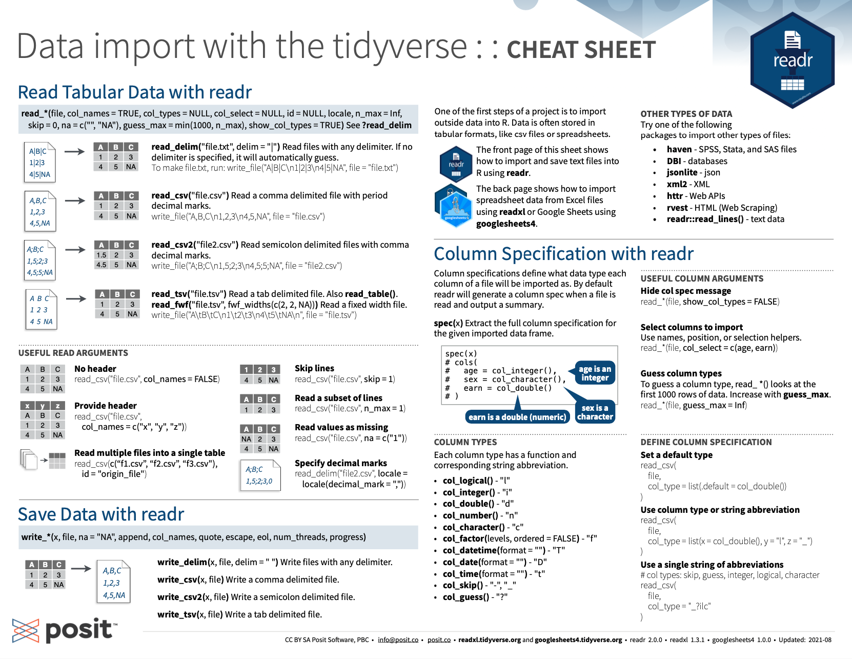
Figure 11.4: The RStudio cheatsheet on importing and exporting data with the readr package.
11.4.3 Preview
In the following Chapter 12 on Using tibbles, we will take a closer look on the tibble package (Müller & Wickham, 2023) that provides the main data structure of the tidyverse (Wickham, 2023b).
11.5 Exercises

Most of the following exercises link to the corresponding exercises of Chapter 6: Importing data.
Please complete at least one exercise of each part (A and B).
11.5.2 Including images by absolute vs. relative links
Suppose you wanted to include an online image in your R Markdown file. To achieve this, you could either
- link to the online image by using its absolute path (to some web server), or
- copy the image into an
/imagesub-directory of your project and use the (absolute or relative) link to this location.
- copy the image into an
Discuss the advantages and disadvantages of both options.
Implement both options for an example image.
Part B: Reading and writing data
The following exercises link to Chapter 6: Importing data of the ds4psy book (Neth, 2023a). To practice importing external data files of various formats, some text files are stored at rpository.com.