20 Basic simulations

The Sims is a successful series of a real-life simulation games. In this game, players can create a virtual character (called a “Sim”), equip it with personality traits and stuff like clothes and furniture, meet friends and foes, and then spend days or weeks by observing and nurturing their artificial alter egos to lead their lives in a simulated environment (Figure 20.1).

Figure 20.1: The Sims Social is a real-life simulation game in which people customize and nurture artificial alter egos and observe and influence their behavior. (Image from EA: The Sims.)

This chapter on Basic simulations is the first chapter in the more general part on Modeling. As our goal is to learn how R can be used for representing and solving problems, we will first concentrate on basic and straightforward simulations that either enumerate cases (in Section 20.2) or sample random values from some distribution (in Section 20.3). While the problems considered here are simple enough that they could still be solved analytically, implementing them familiarizes us with many interesting aspects of computer simulations and provides us with an excellent excuse to solve some entertaining puzzles.

The next Chapter 21 on Dynamic simulations will go beyond these elementary cases to include more complex simulations in which future states and outcomes are harder to anticipate.

Preparation

Recommended background readings for this chapter include:

• Chapters 22: Introduction and 23: Model basics of the r4ds book (Wickham & Grolemund, 2017).

Preflections

Remember that the chapters on simulations are enclosed in a book part that is entitled Modeling. This raises some interesting questions:

• What is a simulation?

• What are the goals of creating a simulation?

• What are the differences of simulation to a model? Specifically,

  • Are all simulations models?
  • Are all models simulations?

20.1 Introduction

Economic simulation games (see Wikipedia) promise to practice skills in a playful setting. Importantly, the conditions and actions of players are processed by rules to yield plausible consequences and outcomes. To be both believable and instructive, such games need to contain a modicum of truth (Figure 20.2).

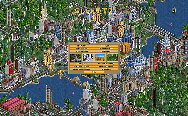
Figure 20.2: OpenTTD is an open source simulation game. (Image from OpenTTD.org.)

Clarify some key terminology. Some concepts that are relevant in the present contexts are:

• the distinction between simulations and modeling,
• situations under risk vs. under uncertainty,
• solving problems by description vs. by experience.

20.1.1 What are simulations?

According to Wikipedia, a computer simulation is the process of running a model. Thus, it does not make sense to “build a simulation”. Instead, we can “build a model”, and then either “run the model” or “run a simulation”.

Despite this agreement, people also call a collection of coded assumptions and rules a simulation, rendering the boundaries between models and simulations blurry again. For our purposes, simulations simply are particular types of models of a situation. Thus, all simulations are models, but there are models (e.g., a mathematical formula) that we would not want to call a simulation.

Conceptually, simulations create concrete observations (i.e., data/cases) from a more abstract description of a problem, task, or situation. Note that, in data analysis, we typically do the reverse: We start with data (concrete observations) and create a more abstract description of the data.

Creating a simulation typically requires that we represent both a situation and the actions or rules specified in a problem description. Conceptually, a representation involves (a) mapping the essential elements of a problem to corresponding elements in a model, and (b) specifying the processes that can operate upon both sets of elements. Once these representational constructs are in place, we can run the simulation repeatedly to observe what happens.

If the description contains probabilistic parameters, the simulation can include random elements. In many contexts, the term “simulation” is used when models contain random elements. For instance, in statistical simulations, we often start by drawing random values from some well-defined distribution and then compute the result of some algorithm based on these values.

Goals of simulations

Creating simulations typically serves two inter-related purposes:

1. Explicate premises and processes: If we cannot solve a problem analytically (e.g., mathematically), we can simulate it to inspect its solution. By implementing both the premises and a mechanism, they explicate the assumptions and consequences of a theory. Often we may notice details or hidden premises that remained implicit or unspecified in the problem formulation.

2. Generate possible results (outputs): This method can be used to explore the consequences of a set of rules or regularities. Such simulations are instantiations that show what happens if certain starting conditions are met and some mechanism is executed. Changing premises or parts of the process shows how this affects our results.

Mental vs. silicon simulations

The idea of using a model or simulation for predicting outcomes is not new — and has often been viewed as an analogy for human thinking, reasoning, and problem solving (see e.g., Craik, 1943; Gentner & Stevens, 1983; Johnson-Laird, 1983). However, rather than thinking things through in our minds, we now also have the computing capacities and tools for quickly building quite powerful computer simulations (e.g., in simulating entire ecosystems or climate phenomena). But out-sourcing simulations from our brains to computing machines does not free us from thinking. The bigger and more complex our simulations get, the more important are solid programming skills and a sound reflection of their pitfalls and limitations.

Crutches vs. useful tools

Note that simulations are often portrayed as a poor alternative to analytic solutions. When we lack the (formal, e.g., mathematical) means to solve something in an analytic fashion, we can use simulations as a crutch that generates results without gaining a clear conceptual and theoretical understanding of the process. However, simulations can also be used in a sensible and responsible fashion (e.g., by systematically varying inputs) and explore systems or theories that are (currently?) too complex to be tackled by analytic approaches (e.g., interactions between neurons in a brain, or sets of physical laws jointly governing weather or climate phenomena). As the merits of any method generally depends on its uses and the availability of alternative approaches, we should generally welcome simulations as one possible way for solving problems.

20.1.2 Static simulations

This chapter on basic simulations focuses on static situations: The environment and the range of moves or options is fixed by the problem description. All relevant information (e.g., the rules of the game or scope of actions) is known a priori.

Such situations can be well-defined, but still contain probabilisitc elements. The psychology of judgment and decision making refers to such situations as risky choice or decision making under risk. A typical situation under risk is repeatedly throwing a random device (e.g., a coin or dice). Here, the set of all possible outcomes and their probabilities can be defined (e.g., by description) or measured (e.g., by experiencing a series of events). Although any particular outcome cannot be know in advance, we can still make observations and predictions regarding the long-term development of outcomes. The mathematics of such problems are governed by the axioms and calculus of probability theory.

By contrast, situations are considered to be under uncertainty when either the set of possible outcomes or their probabilities cannot be known in advance. Most real-life situations are actually under uncertainty, rather than under risk [see Gigerenzer (2014); or Neth & Gigerenzer (2015); for examples]. The boundaries between situations under risk and those under uncertainty are often blurred, as they partly depend on our ability of capturing, expressing, and defining the relevant elements. When considering more complex phenomena (e.g., systems that contain interactions between one or more agents and a reactive and responsive environment), all aspects of a situation may technically still be under risk, yet their dynamic interplay can get too messy and intransparent to provide an analytic solution to the problem. Thus, while analytic solutions may always be desirable, creating simulations may be our only realistic options for keeping track of such environments, their agent(s), or both. (We will examine such situations in Chapter 21 on Dynamic simulations.)

However, even static situations in which the range of optios and probabilities is relatively small and well-defined can often get complex and complicated. Experts in probability may be able to solve them analytically, but the rest of us can tackle them by running a simulation.

For simulating risky situations, we must address the following general issues:

• Creating data structures for representing environments and events
  
• Keeping track of environmental states, actions, and outcomes
  
• Managing sampling processes (i.e., randomness and iterations)

20.1.3 Overview

Conceptually, simulations create concrete observations (i.e., cases or data) from a more abstract description. If this description contains probabilistic parameters, the simulation can include random elements.

In the following, we introduce two basic types of simulations:

1. Enumerating cases essentially explicates information that is contained in a problem description. This most basic type of simulation will be used to illustrate so-called “Bayesian situations”, like the notorious mammography problem (Eddy, 1982, see Section 20.2).

2. Sampling cases employs controlled randomness for solving probabilistic problems by repeated observations. This slightly more sophisticated type of simulation is use to illustrate the Monty Hall problem (Savant, 1990, see Section 20.3).

Conceptually, both types of simulations exploit the continuum between a probabilistic description and its frequentist interpretation as the cumulative outcomes of many repeated random events. As our examples and the exercises (in Section 20.5) will show, the details of the assumed premises and processes matter for the outcomes that we will find — and simulations are particularly helpful for explicating implicit premises and processes.

Problems considered

Examples of problems that can be “solved” by basic simulations include:

• Bayesian situations, like the mammography problem (Eddy, 1982) or cab problem (Kahneman & Tversky, 1972a)
  
• so-called cognitive illusions, like the engineer/lawyer problem or Linda problem; (e.g., Tversky & Kahneman, 1974)
  
• notorious brain teasers, like the Monty Hall dilemma (Savant, 1990; Selvin, 1975) or the three prisoners problem (e.g., Bar-Hillel, 1980)
• other mathematical (Dudeney, 1917) or probability puzzles (Gardner, 1988; Mosteller, 1965), and
• alleged biases in the human perception of randomness (Hahn & Warren, 2009; Kahneman & Tversky, 1972b)

The prominence of this list shows that simulations can address a substantial proportion of the problems discussed in the psychology of human judgment and decision making.

General goals

By implementing these problems, we pursue some general goals that reach beyond the details of any particular problem. These goals include:

1. Explicating a problem’s premises and structure (by implementing it)
   
2. Solving the problem (by repeatedly simulating its assumed process)
3. Evaluating the solution’s uncertainty or robustness (e.g., its variability)

Additional motivations for running simulations are that they can provide new insights into a problem and be a lot of fun — but that partly depends on your idea of fun, of course.

20.2 Enumerating cases

The simplest type of simulation merely explicates information that is fully contained in a problem description. This promotes insight by showing the consequences of premises.

20.2.1 Bayesian situations

For several decades, the psychology of reasoning and problem solving has been haunted by a class of problems. The drosophila task of this field is the so-called mammography problem (based on Eddy, 1982).

The mammography problem

The following version of the mammography problem stems from Gigerenzer & Hoffrage (1995) (using the standard probability format):

1. The probability of breast cancer is 1% for a woman at age forty who participates in routine screening.

2. If a woman has breast cancer, the probability is 80% that she will get a positive mammography.

3. If a woman does not have breast cancer, the probability is 9.6% that she will also get a positive mammography.

A woman in this age group had a positive mammography in a routine screening.
What is the probability that she actually has breast cancer?

Do not despair when you find this problem difficult. Only about 4% of naive people successfully solve this problem (McDowell & Jacobs, 2017).

20.2.2 Analysis

We should first identify precisely what is given and asked in this problem:

What is given?

Identifying the information provided by the problem:

1. Prevalence of the condition (cancer) \(C\): \(p(C)=.01\)

2. Sensitivity of the diagnostic test \(T\): \(p(T|C)=.80\)

3. False positive rate of the diagnostic test \(T\): \(p(T|¬C)=.096\)

What is asked?

Identifying the question: What would solve the problem?

• The conditional probability of the condition, given a positive test result. This is known as the test’s positive predictive value (PPV): \(p(C|T)=?\).

Bayesian solution

The problem provides an unconditional (\(p(C)\)) and two conditional probabilities (\(p(T|C)\) and \(p(T|¬C)\)) and asks for the inverse of one conditional probability (i.e., \(p(C|T)\)). Problems of this type are often framed as requiring ``Bayesian reasoning’’, as their mathematical solution can be derived by a formula known as Bayes’ theorem:

\[ p(C|T) = \frac{p(C) \cdot p(T|C) } {p(C) \cdot p(T|C)~+~p(\neg C) \cdot p(T|\neg C) } = \frac{.01 \cdot .80 } { .01 \cdot .80 ~+~ (1 - .01) \cdot .096 } \approx\ 7.8\%. \]

This looks (and is) pretty complicated — and it’s not surprising that hardly anyone solves the problem correctly.

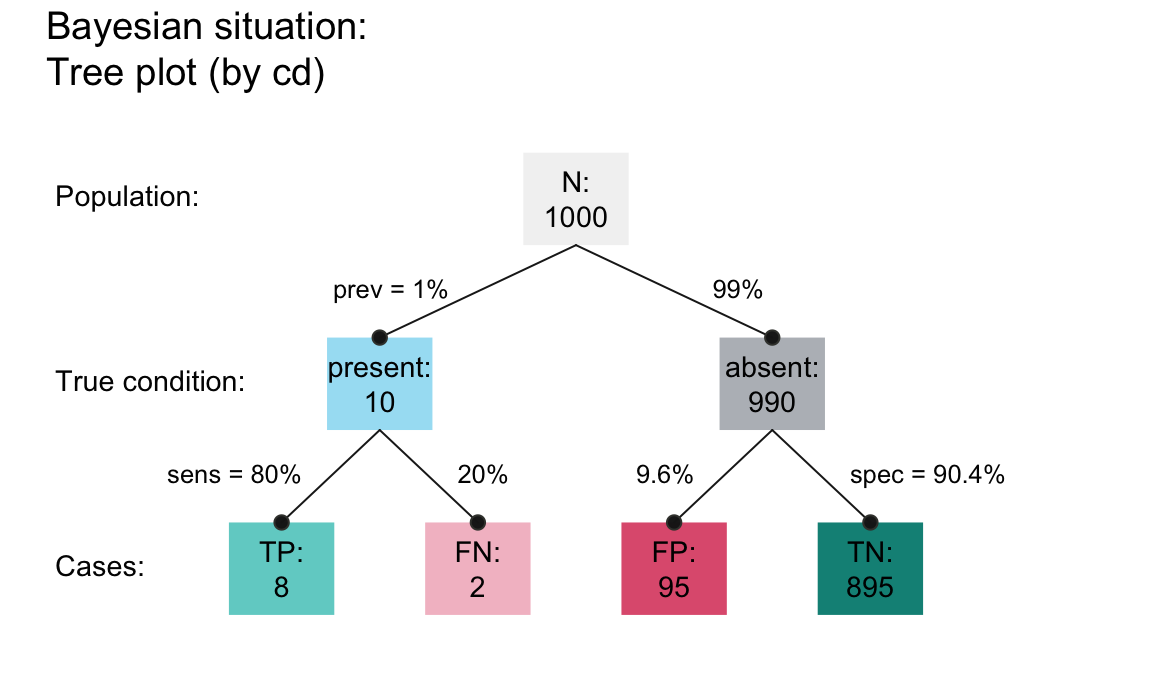
Fortunately, there are much simpler ways of solving this and related problems. Perhaps the most well-known account of so-called “facilitation effects” is provided by Gigerenzer & Hoffrage (1995). The following simulation essentially implements a version of the problem that expresses the probabilities provided by the problem in terms of natural frequencies for a population of \(N\) individuals. This will allow us to replace complex probabilistic calculations by simpler enumerations of cases.

20.2.3 Solution by enumeration

A first approach assumes a population of N individuals and applies the given probabilities to them. We can then inspect the population to derive the desired result.

All fixed, no sampling:

# Parameters:
N <- 1000     # population size
prev <- .01   # condition prevalence
sens <- .80   # sensitivity of the test
fart <- .096  # false alarm rate of the test (i.e., 1 - specificity)

Prepare data structures: Two vectors of length N:

# Prepare data structures:
cond <- rep(NA, N)
test <- rep(NA, N)

Using the information given to compute the expected values (i.e., the number of corresponding individuals if those probabilities are perfectly accurate):

# Compute expected values: 
n_cond <- round(prev * N, 0) 
n_cond_test <- round(sens * n_cond, 0)
n_false_pos <- round(fart * (N - n_cond), 0)

Note that we needed to make two non-trivial decisions in computing the expected values:

• Level of accuracy: Rounding to nearest integers
• Priority: Using value of n_cond in other computations ensures consistency (but also dependencies)

Using these numbers to categorize a corresponding number of elements of the cond and test vectors:

# Applying numbers to population (by subsetting): 

# (a) condition:
cond[1:N] <- "healthy"
if (n_cond >= 1){ cond[1:n_cond] <- "cancer" }
cond <- factor(cond, levels = c("cancer", "healthy"))

# (b) test by condition == "cancer":
test[cond == "cancer"] <- "negative"
if (n_cond_test >= 1) {test[cond == "cancer"][1:n_cond_test] <- "positive"}

# (c) test by condition == "healthy":
test[cond == "healthy"] <- "negative"
if (n_false_pos >= 1) {test[cond == "healthy"][1:n_false_pos] <- "positive"} 
test <- factor(test, levels = c("positive", "negative"))

Analogies:

The following visualizations use the riskyr package (Neth et al., 2022):

• Drawing a tree of natural frequencies:

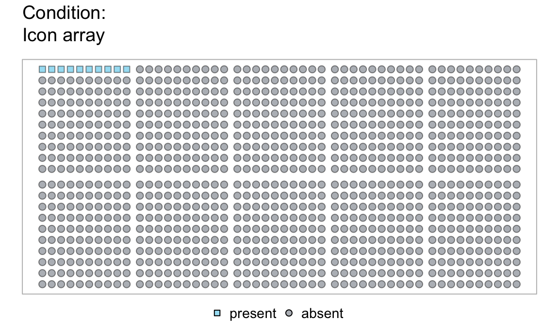
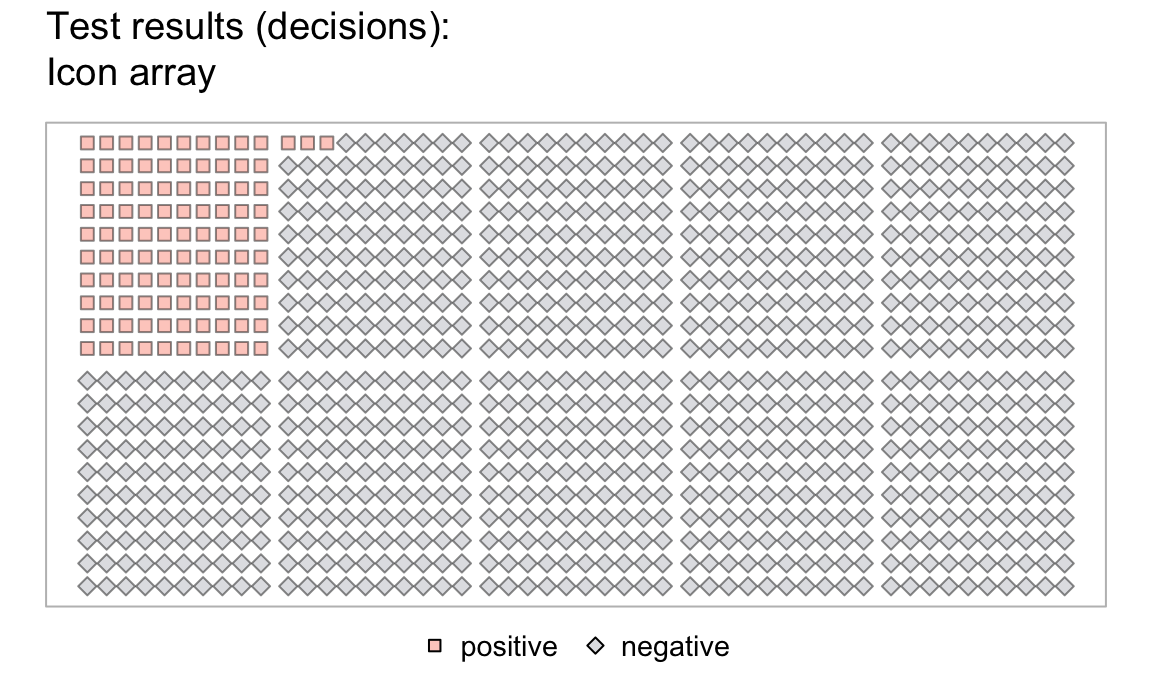
Visualizing the individual items of the population:

• Coloring the N squares of an icon array in three steps:

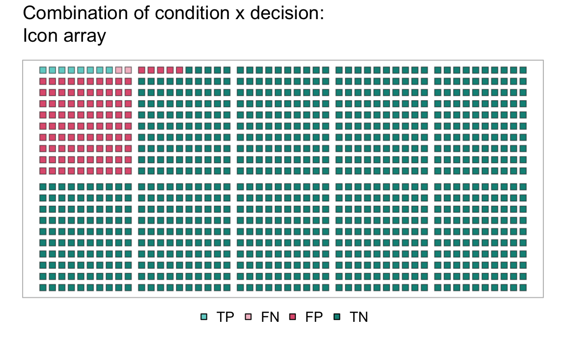
Our result are two vectors (cond and test) with binary categories, which now can be inspected.

Conduct some checks:

# Checks: Are the categories exhaustive?
sum(cond == "cancer")   + sum(cond == "healthy")  == N
#> [1] TRUE
sum(test == "positive") + sum(test == "negative") == N
#> [1] TRUE

# Crosstabulation:
table(test, cond)
#>           cond
#> test       cancer healthy
#>   positive      8      95
#>   negative      2     895

Answer by inspecting table (or the combination of vectors):

sum(test == "positive" & cond == "cancer")  # frequency of target individuals
#> [1] 8
sum(test == "positive" & cond == "cancer") / sum(test == "positive")  # desired conditional probability
#> [1] 0.0776699

Note that this solution used the probabilistic information, but required no random or statistical processes. Instead, we assumed a large population of N individuals and used the probabilities to enumerate the corresponding number (or proportions) of individuals in subgroups of the population. The resulting proportion of individuals who both test positive and suffer from cancer out of those with a positive test result matches our analytic solution of \(p(C|T) = 7.8\%\) from above.

An alternative way of solving this problem could take probability more seriously by adding random sampling. We will leave this to Exercise 20.5.4, but use a different problem to illustrate sampling-based simulations (in Section 20.3).

20.2.4 Visualizing Bayesian situations

The following visualizations further illustrate the solutions for the Bayesian situation of the mammography problem that was derived in this section:

• A frequency net (Binder et al., 2020) provides an overview of the subsets of frequencies (as nodes) and the probabilities (as edges between nodes):

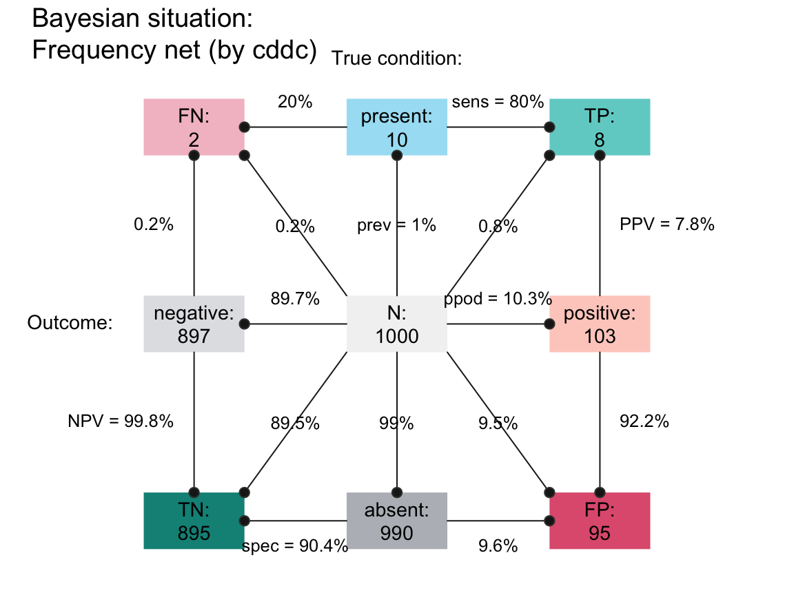
• The same information can be expressed in two distinct frequency tree diagrams:

The visualizations shown here use the riskyr package (Neth et al., 2022). See Neth et al. (2021) for the theoretical background of such problems.

20.3 Sampling cases

Goal: Taking probabilities more seriously by actually using the probabilities provided in a process of random sampling. This adds complexity (e.g., different runs yield different outcomes) but may also increase the realism our our simulation (as it’s unlikely to obtain perfectly stable results in reality).

Rather than calculate the expected values, we use the probabilities stated in the problem to sample from the appropriate population.

Two important aspects of managing randomness:

• Use set.seed() for reproducible randomness.
• Assess the robustness of results based on repetitions.

20.3.1 The Monty Hall problem

A notorious brain teaser problem is based on the US-American TV show Let’s make a deal (see Selvin, 1975). The show involves that a lucky player faces a choice between three doors. It is known that one door hides the grand prize of a car (i.e., win), whereas the other two hide goats (i.e., losses). After choosing a closed door (e.g., Door 1), the show’s host (named Monty Hall) intervenes by opening one of the unchosen doors to reveal a goat. He then offers the player the option to switch to the other closed door. Should the player switch to the other door? The player’s situation is illustrated by Figure 20.3.

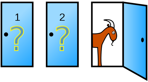
Figure 20.3: The Monty Hall problem from the player’s perspective. (Source: Illustration from Wikipedia: Monty Hall problem.)

The problem

The following version of the dilemma was famously discussed by Savant (1990):

Suppose you’re on a game show, and you’re given the choice of three doors:
Behind one door is a car; behind the others, goats.
You pick a door, say No. 1, and the host, who knows what’s behind the doors,
opens another door, say No. 3, which has a goat.
He then says to you, “Do you want to pick door No. 2?”
Is it to your advantage to switch your choice?

Note that the correct answer to the question asked is either “yes” or “no”. Answering “yes” implies that switching doors is generally better than staying with the initial choice. By contrast, answering “no” implies that staying is generally at least not worse than switching doors.

20.3.2 Analysis

This problem and its variants have been widely debated — and even revealing its solution is often met with disbelief and likely to spark controversy.

Most people intuitively assume that — given Monty Hall’s intervention — the player faces a 50:50 chance of winning and it therefore makes no difference whether she sticks with her initial choice or switches to the other door. (Note that this does not yet justify why the majority of people prefer to stick with their initial door, but we could postulate a variety of so called “biases” or psychological mechanisms for this preference.)

However, the correct answer to the question is “yes”: The player is more likely to win the car if she always switches to the alternative door. There are many possible ways to explain this:

• Perhaps the simplest explanation asks: What is the probability of winning the car with the player’s initial choice (i.e., without any other interactions)? Most people would agree that \(p(win\ with\ d_i) = \frac{1}{3}\) for any arbitrary door \(d_i\). Accepting that Monty Hall’s actions cannot possibly change this (as he cannot transfer the car to a different location), we should conclude that the winning chance for sticking with the initial choice also is \(p(stay) = \frac{1}{3}\) and \(p(switch) = 1 - p(stay) = \frac{2}{3}\). (The subtle reason for the benefit for switching is that Monty Hall must take the car’s location into account to reliably open a door that reveals a goat. Thus, Monty Hall curates the choices in a way that adds information.)

• A model-based approach could visualize the three possible options for the car’s location (which are known to be equiprobable, given the car’s random allocation). By explicating the consequences of an initial choice (e.g., of Door 1), we see that always sticking with the initial choice has a theoretical chance of winning in \(p(stay) = \frac{1}{3}\) of cases. By contrast, always switching to the alternative door provides a higher change of winning of \(p(switch) = \frac{2}{3}\) (see Figure 20.4).

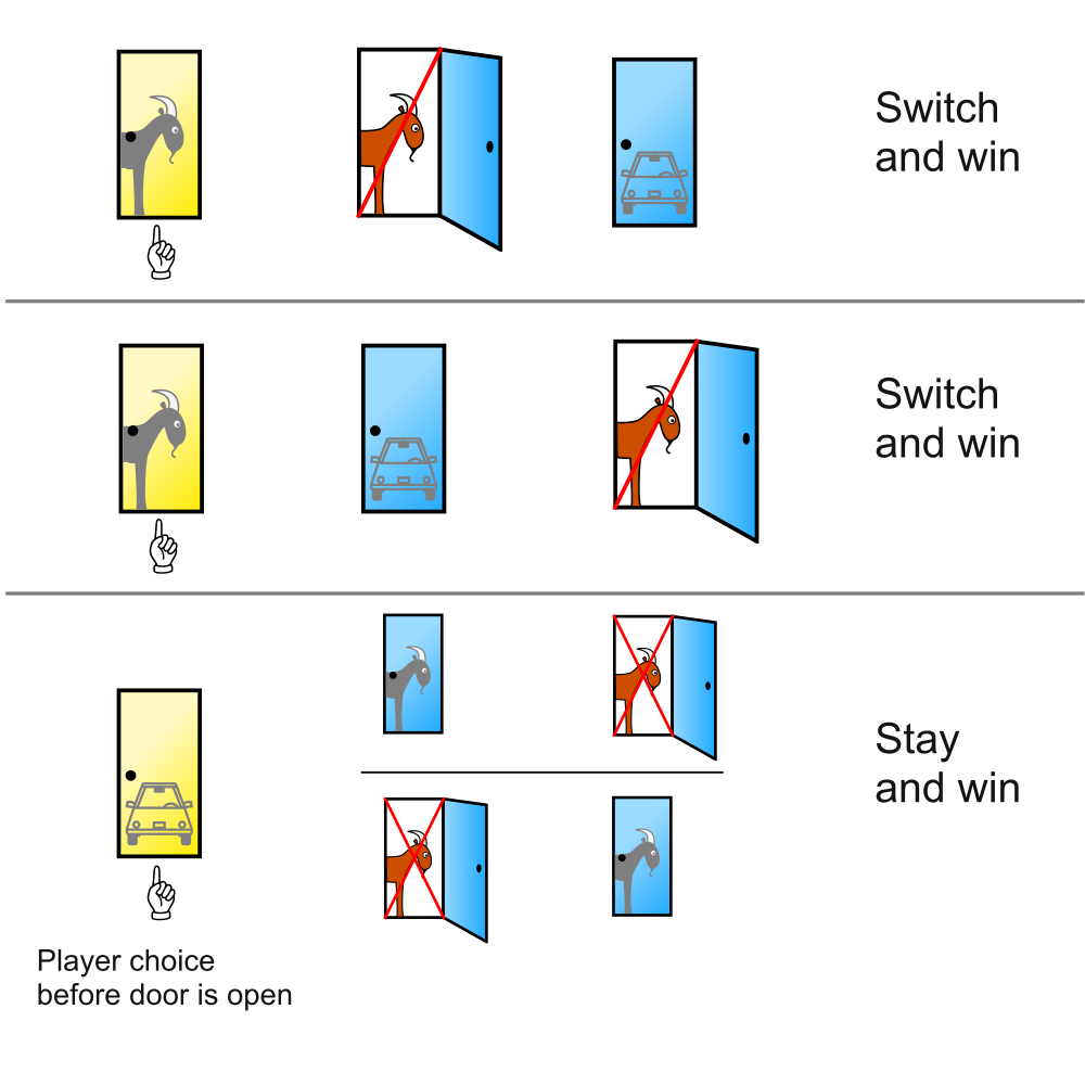
Figure 20.4: An explanation for the superiority of switching in the Monty Hall problem. (Source: Illustration from Wikipedia: Monty Hall problem.)

Many people find the correct solution so counterintuitive that they are unwilling to accept these explanations. If someone refuses to accept the theoretical arguments, an alternative way of convicing them is by simulating a large number of games and then compare the success of either staying or switching doors.²⁹

20.3.3 Representing the environment

Our task is to use simulations to decide and justify whether the the contestant should stay or switch. More precisely, is the probability of winning the game by switching larger than by staying with the initial door? What are the probabilities for winning the car in both cases?

To solve this task, we create a simulation with the following features: 3 doors, random location of the car, Monty knows the car’s location and always opens a door that reveals a goat. (Exercise 20.5.5 will extend this solution to some variants of the problem.)

Preparations

The most important element for any simulation is to create a valid model of the game scenario.

We will first create a data structure that can represent the setups for N games:

# Generate a random setup:
setup <- sample(x = c("car", "goat", "goat"), size = 3, replace = FALSE)
setup
#> [1] "goat" "car"  "goat"

# Create N games (with a column for each door):
N <- 100
games <- NA

# Prepare data structure: 
games <- tibble::tibble(d1 = rep("NA", N),
                        d2 = rep("NA", N),
                        d3 = rep("NA", N))

Sampling setups

We now create N random setups and store them in our prepared table of games:

# Fill table with random games:
set.seed(2468)  # for reproducible randomness

for (i in 1:N){
  
  setup <- sample(x = c("car", "goat", "goat"), size = 3, replace = FALSE)
  
  games$d1[i] <- setup[1]
  games$d2[i] <- setup[2]
  games$d3[i] <- setup[3]
  
}

head(games)
#> # A tibble: 6 × 3
#>   d1    d2    d3   
#>   <chr> <chr> <chr>
#> 1 goat  car   goat 
#> 2 goat  goat  car  
#> 3 car   goat  goat 
#> 4 goat  goat  car  
#> 5 car   goat  goat 
#> 6 goat  goat  car

Note on set.seed(2468): ensure reproducible randomness. Any value is fine, in principle, but avoid always using the same values. Importantly, using unconstrained randomness can often be a virtue!

20.3.4 Abstract solution

Our first simulation of the problem is rather abstract insofar as it ignores all details of Monty’s actions.
When realizing that the game show host (named Monty) can always open a door with a goat (since there are two of them), we can simulate the outcome of the game without taking his actions into account.

We first create an auxiliary function that allows us to determine whether a game has been won. This depends on the contents of the three doors (i.e., the car’s location) and the player’s final choice (i.e., of Door 1, 2, or 3). A game is won whenever the chosen door contains the car:

# Given the specific setup of a game, would the chosen door win the car? 
win_car <- function(d1, d2, d3, choice){
  
  out <- FALSE
  setup <- c(d1, d2, d3)
  
  if (setup[choice] == "car"){
    out <- TRUE
  }
  
  return(out)
  
}

# Check:
win_car("car", "goat", "goat", 1) 
#> [1] TRUE
win_car("car", "goat", "goat", 2)
#> [1] FALSE
win_car("car", "car", "goat",  2)
#> [1] TRUE
win_car("car", "car", "goat",  3)
#> [1] FALSE

Simulate the outcomes of N games in three steps:

1. Generate N initial door choices:

As the player’s initial choices are independent of the game’s setup, we can either always pick the same door (e.g., Door 1) or select a random door (i.e., 1, 2, or 3) in each game. As picking a random door in each game appears more plausible, we use sample() to draw N initial choices and add those as a new variable to games:

# 1. Generate and add N initial door choices:
sim_1 <- games %>%
  mutate(init_door = sample(x = 1:3, size = N, replace = TRUE))

Several details of this step are noteworthy:

• Our mutate() function to compute init_door (in Step 1.) contained a second call to sample(), but always picking Door 1 should make no difference for the result, as long as each row of games really was created randomly above.³⁰

• In this call to sample(), we specified replace = TRUE to ensure that repeatedly drawing the same door is possible and that sampling \(N>3\) times from x = 1:3 is possible.

• As we set set.seed(2468) above, the first call this instance of sample() will always yield the same sequence of results. However, as we did not fix a new value of set.seed() here, repeating this step multiple times would create different values every time.

2. Determine all wins by staying:

Given a specific setup of doors and the player’s initial choice, we can determine whether staying with the initial choice would win the car:

# 2. Determine wins by staying: 
sim_1 <- sim_1 %>%
  mutate(win_stay = purrr::pmap_lgl(list(d1, d2, d3, init_door), win_car))

Note: An example for different map() functions of the purrr package:

# Functions:
square <- function(x){ x^2 }
expone <- function(x, y){ x^y }

# Data:
tb <- tibble(n_1 = sample(1:9, 100, replace = TRUE),
             n_2 = sample(1:3, 100, replace = TRUE))

# map functions to every row of tb:
tb %>% 
  mutate(sqr = purrr::map_dbl(.x = tb$n_1, .f = square),  # 1 argument
         exp = purrr::map2_dbl(n_1, n_2, expone),         # 2 arguments
         sum = purrr::pmap_dbl(list(n_1, n_2, sqr), sum)  # 3+ arguments
         )
#> # A tibble: 100 × 5
#>     n_1   n_2   sqr   exp   sum
#>   <int> <int> <dbl> <dbl> <dbl>
#> 1     1     2     1     1     4
#> 2     9     1    81     9    91
#> 3     3     3     9    27    15
#> 4     2     3     4     8     9
#> 5     4     1    16     4    21
#> 6     9     3    81   729    93
#> # … with 94 more rows
#> # ℹ Use `print(n = ...)` to see more rows

3. Determine all wins by switching:

The third and final step may require some explanation: Assuming that Monty knows the car’s location, but always opens a door with a goat, we can conclude that switching doors wins the game in exactly those cases in which the player’s initial choice did not win the game. A simpler way of expressing this is: Switching doors wins the game whenever the initial choice does not succeed.

# 3. Determine wins by switching: 
sim_1 <- sim_1 %>%
  mutate(win_switch = !win_stay)

Note that we could combine the three steps above in a single mutate() command:

sim_1 <- games %>%
  mutate(init_door = sample(1:3, N, replace = TRUE), 
         win_stay = purrr::pmap_lgl(list(d1, d2, d3, init_door), win_car), 
         win_switch = !win_stay)

4. Evaluate results:

At this point sim_1 contains all the information that we need. For instance, to compare the result of consistently staying or switching, we simply inspect the final two variables:

head(sim_1)
#> # A tibble: 6 × 6
#>   d1    d2    d3    init_door win_stay win_switch
#>   <chr> <chr> <chr>     <int> <lgl>    <lgl>     
#> 1 goat  car   goat          1 FALSE    TRUE      
#> 2 goat  goat  car           3 TRUE     FALSE     
#> 3 car   goat  goat          3 FALSE    TRUE      
#> 4 goat  goat  car           1 FALSE    TRUE      
#> 5 car   goat  goat          3 FALSE    TRUE      
#> 6 goat  goat  car           2 FALSE    TRUE

# Results for staying vs. switching: 
mean(sim_1$win_stay)
#> [1] 0.32
mean(sim_1$win_switch)
#> [1] 0.68

As our theoretical analysis has shown, always switching turns out to be about twice as good as always sticking to the initial choice.

20.3.5 Detailed solution

A more concrete simulation would also incorporate the details of Monty’s actions:

Note that we can select game setups and determine the locations of the car and goats as follows:

setup <- games[1, ]  # select a specific setup (row in games)
setup

# Determining locations of interest:
which(setup == "car")  # car's location/index
which(setup == "goat") # goat locations

To flesh out the details of a particular game, we first need to create two additional auxiliary functions:

1. Simulate Monty’s actions (i.e., which door is being opened, based on the setup and the player’s initial choice):

# 1. Monty acts as a function of current setup and player_choice: 
host_act <- function(d1, d2, d3, player_choice){
  
  door_open <- NA
  setup <- c(d1, d2, d3)
  ix_goats <- which(setup == "goat")  # indices of goats
    
  # Distinguish 2 cases:
  if (setup[player_choice] == "car"){ # player's initial choice would win the car:
    
    door_open <- sample(ix_goats, 1)  # show a random goat (without preference)
    
  } else { # player's initial choice is a goat: 
    
    door_open <- ix_goats[ix_goats != player_choice]  # show the other/unchosen goat
    
  }
  
  return(door_open)
  
}

# Check:
host_act("car", "goat", "goat", 2)  # Monty must open d3
#> [1] 3
host_act("car", "goat", "goat", 3)  # Monty must open d2
#> [1] 2
host_act("car", "goat", "goat", 1)  # Monty can open d2 or d3
#> [1] 2
host_act("car", "goat", "goat", 1)  # Monty can open d2 or d3
#> [1] 3

Note that we enter the contents of the three doors as three distinct arguments (i.e., d1, d2, and d3), rather than as one argument that uses the vector setup. The reason for this is that we later want to use entire rows of games as inputs to the map() family of functions of the purrr package.

2. Identify the door to switch to (based on an initial choice and Monty’s actions):

# 2. To which door would the player switch (based on initial choice and Monty's action): 
switch_door <- function(door_init, door_open){
  
  door_switch <- NA
  doors <- 1:3
  
  door_switch <- doors[-c(door_init, door_open)]

  return(door_switch)
  
}

# Check:
switch_door(1, 2)
#> [1] 3
switch_door(1, 3)
#> [1] 2
switch_door(2, 1)
#> [1] 3
switch_door(2, 3)
#> [1] 1
switch_door(3, 1)
#> [1] 2
switch_door(3, 2)
#> [1] 1

3. Simulate N games:

Equipped with these functions, we can now generate all details of N games as a single dplyr pipe:

sim_2 <- games %>%
  mutate(door_init = sample(1:3, N, replace = TRUE),  # sample initial choices
         # door_init = rep(1, N),  # (always pick Door 1 as initial choice)  
         # door_init = sim_1$init_door,  # (use the same choices as above)
         door_host = purrr::pmap_int(list(d1, d2, d3, door_init), host_act),
         door_switch = purrr::pmap_int(list(door_init, door_host), switch_door),
         win_stay = purrr::pmap_lgl(list(d1, d2, d3, door_init), win_car),
         win_switch = purrr::pmap_lgl(list(d1, d2, d3, door_switch), win_car)
         )
head(sim_2)
#> # A tibble: 6 × 8
#>   d1    d2    d3    door_init door_host door_switch win_stay win_switch
#>   <chr> <chr> <chr>     <int>     <int>       <int> <lgl>    <lgl>     
#> 1 goat  car   goat          3         1           2 FALSE    TRUE      
#> 2 goat  goat  car           2         1           3 FALSE    TRUE      
#> 3 car   goat  goat          2         3           1 FALSE    TRUE      
#> 4 goat  goat  car           3         2           1 TRUE     FALSE     
#> 5 car   goat  goat          3         2           1 FALSE    TRUE      
#> 6 goat  goat  car           2         1           3 FALSE    TRUE

4. Evaluate results:

# Results for staying vs. switching: 
mean(sim_2$win_stay)
#> [1] 0.37
mean(sim_2$win_switch)
#> [1] 0.63

As expected, always switching is still about twice as good as always sticking to the initial choice.

20.3.6 Visualizing simulation results

Whenever running a simulation, it is a good idea to visualize its results. To visualize the number of cumulative wins for consistently using either strategy, we first add some auxiliary variables:

# Add game nr. and cumulative sums to sim:
sim_2 <- sim_2 %>%
  mutate(nr = 1:N,
         cum_win_stay = cumsum(win_stay),
         cum_win_switch = cumsum(win_switch))
dim(sim_2)
#> [1] 100  11

Plot the number of wins per strategy (as a step function):

ggplot(sim_2) +
  geom_step(aes(x = nr, y = cum_win_switch), color = Seeblau, size = 1) + 
  geom_step(aes(x = nr, y = cum_win_stay), color = Bordeaux, size = 1) + 
  labs(title = "Cumulative number of wins for staying vs. switching", 
       x = "Game nr.", y = "Sum of wins", 
       caption = paste0("Data from simulating ", N, " games.")) +
  theme_ds4psy()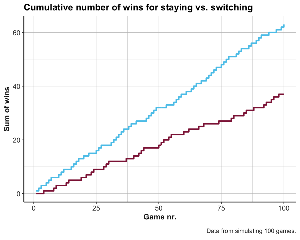

Note that the graph shows that both strategies are indistinguishable at first, but increasingly separate as we play more games. Also, there can be quite long stretches of games for which either strategy fails to win.

Also, the results of our abstract and detailed simulations differ although we used the same setup of games for both. This is because we used sample() to determine the player’s initial choice door_init twice. If we wanted to obtain the same results in both simulations, we could sample the player’s initial choices only once for both simulations or use set.seed() to reproduce the same random sequence twice. However, the variation in results is actually informative. Increasing the number of games N will allow us to approximate the theoretically expected values (of \(p(stay) = \frac{1}{3}\) and \(p(switch) = \frac{2}{3}\)).

Practice

• Explain in your own words why the results for our abstract and detailed solutions slightly differ from each other.

• We decided to let the player choose a random initial door in each game. Confirm that simulating the case in which the player always picks Door 1 would yield the same (qualitative) result.

• Adjust the abstract and detailed simulations so that both allow for random elements (e.g., random game setups and random picks of the player’s initial door), but nevertheless yield exactly the same result.

20.4 Conclusion

20.4.1 Summary

Simulations are a programming technique that force us to explicate premises and processes that are easily overlooked when merely relying on verbal problem descriptions.

In this chapter, we introduced and illustrated two basic types of simulations:

1. by enumeration (explicating the information contained in a problem description)

2. by sampling (involving actual randomness and the need for managing repetitions)

Both types of simulations involve probabilistic information, but deal with it in different ways.

When simulating non-trivial problems with many assumptions, even basic simulations often yield unexpected and surprising results. In addition, simulations often allow to evaluate the robustness of phenomena (e.g., the variability in results due to random sampling).

20.4.2 Resources

Pointers to related sources of inspirations and ideas:

On simulations

• Chapter 20 Simulation (by Peng, 2016) provides a basic introduction into generating random numbers and simple simulations.

On the Monty Hall problem

• Wikipedia: Monty Hall problem summarizes the history and controversy surrounding the problem, and provides pointers to several variants and similar puzzles.

• See Statistics How To: Monty Hall problem for additional links and resources.

• The psychology of the Monty Hall problem is investigated in Krauss & Wang (2003). The problem’s Bayesian structure and reasons for the most common error are explicated in Section 5. Applications of Neth et al. (2021).

• Math 187: Introduction to Cryptography lets you play interactive simulations:

  • Let’s Make a Deal: Monty knows vs.
    
  • Let’s Make a Deal: Monty does not know

20.5 Exercises

The following exercises further explore the interplay between simulations and analytic solutions by examining different types of problems:

• simple mathematical puzzles
• more Bayesian situations
• other versions of the Monty Hall problem
• related probability puzzles

20.5.1 Fun factorials

How many solutions exist for the equation

• \(m! = m^3 – m\)

with \(m\) in \(\mathbb{N}\)?

We can easily conduct a small simulation that solves this problem.

• This puzzle appeared in the “Weekly riddle” column of SPON (Holger Dambeck, 2024-03-31, URL) and the ‘Mr Math11’ YouTube channel.

20.5.2 How many shells in each hand?

A child collects 30 small clam shells on a beach. She holds most of them in her left hand, the others in her right hand. Asked about their number, she responds:

“When I add their number to the square and cube of itself, and do this for both hands, the total amounts to 8058.”

• How many shells does she carry in each hand?

This mathematical puzzle can be solved in a brute force simulation (using loops).
Let’s also keep track of the number of trials we consider:

• How many combinations does our simulation compute?

Notes

• An algebraic solution would require using the binomial formulas
  \((a + b)^{2} = a^2 + 2ab + b^2\) and
  \((a + b)^3 = a^3 + 3a^2b + 3ab^2 + b^3\).

• A version of this puzzle appears in the book Famous puzzles of great mathematicians (2009) by Miodrag S. Petkovic.

20.5.3 More Bayesian situations

The mammography problem shown in Section 20.2 is a special case of a more general class of Bayesian situations, which require the computation of an inverse conditional probability \(p(C|T)\) when given a prior probability \(p(C)\) and two conditional probabilities \(p(T|C)\) and \(p(T|\neg C)\).

In 2021, an intriguing version of this problem is the following: The list of rapid SARS-CoV-2 self tests of the BfArM contains over 450 tests. Each test is characterized by its sensitivity \(p({T+}|infected)\) and specificity \(p({T-}|not\ infected)\). The current local prevalence of SARS-CoV-2 infections (as of 2021-05-20) is 100 out of 100,000 people.

1. Download the table of all tests and compute their mean sensitivity and specificity values.

2. Compute two conditional probabilities:

   • What is the average probability of being infected upon a positive test result (i.e., \(PPV = p(infected|{T+})\)?
   • What is the average probability of not being infected upon a negative test result (i.e., \(NPV = p(not\ infected|{T-})\)?

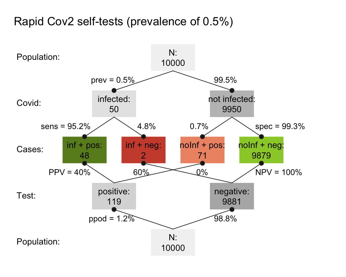
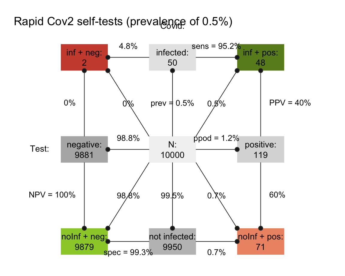
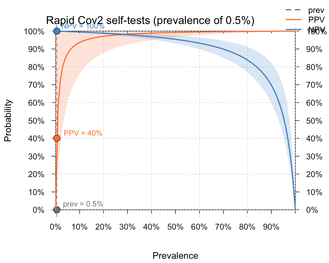
3. How would the values of 2. change, if the local prevalence of SARS-CoV-2 infections rose to 500 out of 100,000 people?

4. Conduct a simulation by enumeration to compute both values for a population of 10,000 people.

5. Bonus: Try visualizing your results (in any way, i.e., not necessarily by using the riskyr package).

Solution

The following table summarizes the mean sensitivity and specificity values of all tests:

Table 20.1: Summary of 455 tests.

n	sens_mean	sens_min	sens_max	sens_sd	spec_mean	spec_min	spec_max	spec_sd
455	95.2191	80.2	100	3.111103	99.28365	96.7	100	0.6847694

The results of 2. and 3. could be computed by the Bayesian formula (see in Section 20.2). The following visualizations result from creating riskyr scenarios.

• Solutions for a prevalence of 100 out of 100,000 people:

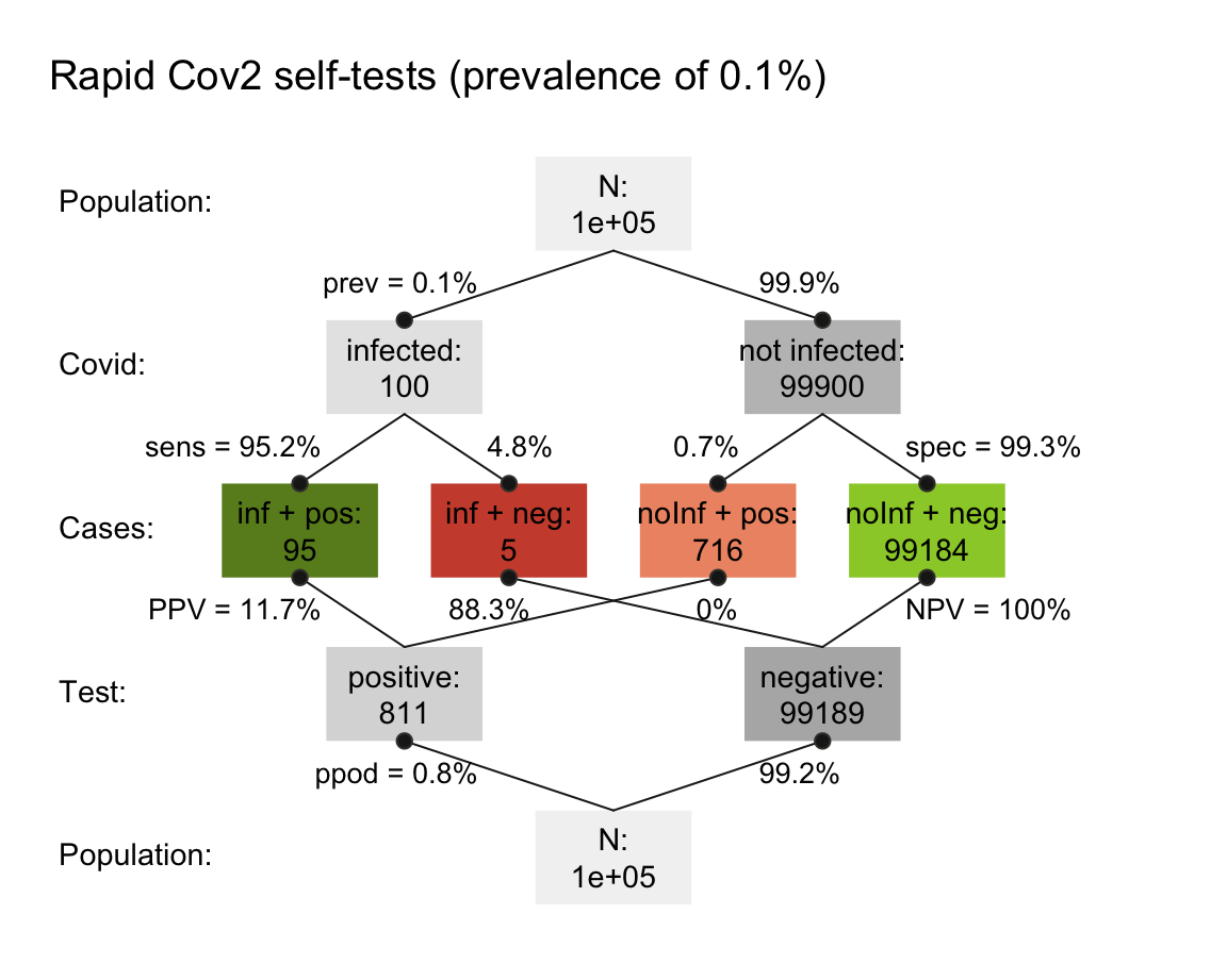
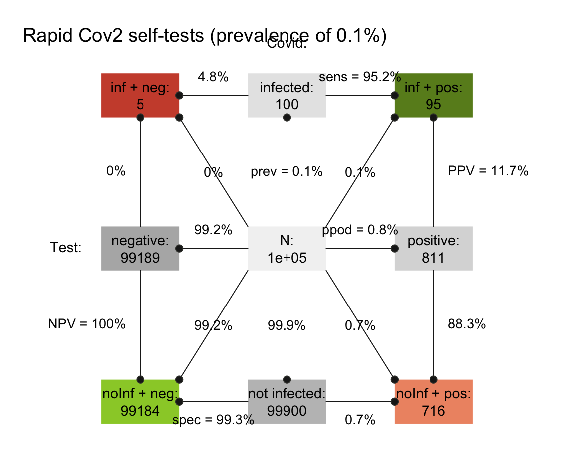
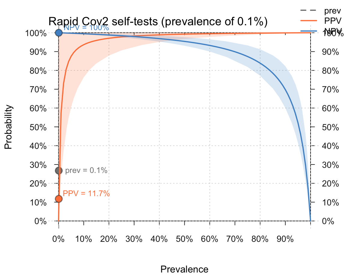
• Solutions for a prevalence of 500 out of 100,000 people:

20.5.4 Solving Bayesian situations by sampling

In Section 20.2, we solved so-called Bayesian situations (and the mammography problem) by enumerating cases. However, we can also use a sampling approach to address and solve such problems.

1. Use a sampling approach for solving the mammography problem (discussed in Section 20.2).

2. Adopt either approach (i.e., either enumeration and sampling) for solving the cab problem (originally introduced by Kahneman & Tversky, 1972a; and discussed by, e.g., Bar-Hillel, 1980):

A cab was involved in a hit-and-run accident at night.
Two cab companies, the Green and the Blue, operate in the city.
You are given the following data:
1. 85% of the cabs in the city are Green and 15% are Blue.
2. A witness identified the cab as a Blue cab.
The court tested his ability to identify cabs under the appropriate visibility conditions. When presented with a sample of cabs (half of which were Blue and half of which were Green) the witness correctly identified each color in 80% of the cases and erred in 20% of the cases.

What is the probability that the cab involved in the accident was Blue rather than Green?

Hint: Despite their superficial differences, the structure of the cab problem is almost identical to the mammography problem (e.g., compare Figures 4 and 9 of Neth et al., 2021).

3. Discuss the ways in which the enumeration and sampling approaches differ from each other and from deriving an analytic solution. What are the demands of each method and the key trade-offs between them?

20.5.5 Monty Hall reloaded

In Section 20.3.1, we introduced the notorious brain teaser known as the Monty Hall dilemma (Savant, 1990; MHD, popularized by Selvin, 1975) and showed how it can be solved by a simulation that randomly samples environmental states (i.e., the setup of games) and actions (e.g., the host’s and player’s choices).

An erroneous MHD simulation

A feature of simulations is that they are only as good as the thinking that created them. And just like statements or scientific theories, they are not immune to criticism, and can be wrong and misleading. In the following, we illustrate this potential pitfall of simulations by creating an enumeration that yields an erroneous result.

So stay alert — and try to spot any errors we make! Importantly, the error is not in the method or particular type of simulation, but in our way of thinking about the problem.

1. Setup

Without considering any specific constraints, the original problem description of the MHD describes a 3x3x3 grid of cases:

• 3 car locations
• 3 initial player picks
• 3 doors that Monty could open

The following tibble grid_MH creates all 27 cases that are theoretically possible:

# Setup of options:
car    <- 1:3
player <- 1:3
open   <- 1:3

# Table/space of all 27 options:
grid_MH <- expand_grid(car, player, open)
# names(grid_MH) <- c("car", "player", "open")

grid_MH <- tibble::as_tibble(grid_MH) %>% 
  arrange(car, player)

grid_MH
#> # A tibble: 27 × 3
#>     car player  open
#>   <int>  <int> <int>
#> 1     1      1     1
#> 2     1      1     2
#> 3     1      1     3
#> 4     1      2     1
#> 5     1      2     2
#> 6     1      2     3
#> # … with 21 more rows
#> # ℹ Use `print(n = ...)` to see more rows

2. Adding constraints

However, not all these cases are possible, as Monty cannot open just any of the three doors. More specifically, the problem description imposes two key constraints on Monty’s action:

• Condition 1: Monty cannot open the door actually containing the car.

• Condition 2: Monty cannot open the door initially chosen by the player.

This allows us to eliminate some cases, or describe which of the 27~theoretical cases are actually possible in this problem:

grid_MH$possible <- TRUE  # initialize

grid_MH$possible[grid_MH$open == grid_MH$car]    <- FALSE  # condition 1
grid_MH$possible[grid_MH$open == grid_MH$player] <- FALSE  # condition 2

grid_MH
#> # A tibble: 27 × 4
#>     car player  open possible
#>   <int>  <int> <int> <lgl>   
#> 1     1      1     1 FALSE   
#> 2     1      1     2 TRUE    
#> 3     1      1     3 TRUE    
#> 4     1      2     1 FALSE   
#> 5     1      2     2 FALSE   
#> 6     1      2     3 TRUE    
#> # … with 21 more rows
#> # ℹ Use `print(n = ...)` to see more rows

3. Eliminating impossible cases

Next, we remove the impossible cases and consider only possible ones (i.e., possible == TRUE):

grid_MH_1 <- grid_MH[grid_MH$possible == TRUE, ]

grid_MH_1
#> # A tibble: 12 × 4
#>     car player  open possible
#>   <int>  <int> <int> <lgl>   
#> 1     1      1     2 TRUE    
#> 2     1      1     3 TRUE    
#> 3     1      2     3 TRUE    
#> 4     1      3     2 TRUE    
#> 5     2      1     3 TRUE    
#> 6     2      2     1 TRUE    
#> # … with 6 more rows
#> # ℹ Use `print(n = ...)` to see more rows

Note that we used base R functions to add a new variable (possible), determine its values (by logical indexing) and then filter its rows (by logical indexing) to leave only possible cases in grid_MH_1.

The following tidyverse solution replaces the last two steps by a simple dplyr pipe (and would have worked without the additional possible variable):

grid_MH_1 <- grid_MH %>%
  filter(open != car, open != player)  # condition 1 and 2

grid_MH_1
#> # A tibble: 12 × 4
#>     car player  open possible
#>   <int>  <int> <int> <lgl>   
#> 1     1      1     2 TRUE    
#> 2     1      1     3 TRUE    
#> 3     1      2     3 TRUE    
#> 4     1      3     2 TRUE    
#> 5     2      1     3 TRUE    
#> 6     2      2     1 TRUE    
#> # … with 6 more rows
#> # ℹ Use `print(n = ...)` to see more rows

ToDo: Visualize the 12 possible cases in a 3x3x3 cube.

4. Determine wins by strategy

Finally, we can determine the number of wins, based on the player’s strategy (i.e., staying with the original choice, or switching to the other remaining door):

• Win by staying: Staying wins whenever the location of the car matches the initial choice of the player.

• Win by switching: As we are only left with possible cases, switching wins whenever staying fails to win.

grid_MH_1$win_stay   <- FALSE  # initialize
grid_MH_1$win_switch <- FALSE

grid_MH_1$win_stay[grid_MH_1$car == grid_MH_1$player] <- TRUE  # win by staying
grid_MH_1$win_switch[grid_MH_1$win_stay == FALSE]     <- TRUE  # win by switching 

grid_MH_1
#> # A tibble: 12 × 6
#>     car player  open possible win_stay win_switch
#>   <int>  <int> <int> <lgl>    <lgl>    <lgl>     
#> 1     1      1     2 TRUE     TRUE     FALSE     
#> 2     1      1     3 TRUE     TRUE     FALSE     
#> 3     1      2     3 TRUE     FALSE    TRUE      
#> 4     1      3     2 TRUE     FALSE    TRUE      
#> 5     2      1     3 TRUE     FALSE    TRUE      
#> 6     2      2     1 TRUE     TRUE     FALSE     
#> # … with 6 more rows
#> # ℹ Use `print(n = ...)` to see more rows

Of course we could have used dplyr mutate() commands, rather than base R indexing to initialize and define these win_stay() and win_switch variables. (We will show a tidyverse solution below.)

5. Count wins by strategy

To compare both strategies, we can now count how often each strategy wins:

# Result*(erroneous): 
(n_win_stay   <- sum(grid_MH_1$win_stay))    # win by staying
#> [1] 6
(n_win_switch <- sum(grid_MH_1$win_switch))  # win by switching
#> [1] 6

6. Interpret solution

This analysis suggests that the chances are 50:50 (or rather 6:6) — which is wrong!

But where is the error? And can we fix this simulation and reach the right solution by enumerating cases?

Analysis: What went wrong?

The previous simulation illustrates a crucial problem with enumerating cases: The cases noted in the reduced grid_MH_1 are not equiprobable (i.e., expected to appear with an equal probability). To see this, let’s take another look at our reduced grid_MH_1:

# Re-inspect grid_MH_1: 
grid_MH_1 %>% filter(car == 1)     # car behind door 1:
#> # A tibble: 4 × 6
#>     car player  open possible win_stay win_switch
#>   <int>  <int> <int> <lgl>    <lgl>    <lgl>     
#> 1     1      1     2 TRUE     TRUE     FALSE     
#> 2     1      1     3 TRUE     TRUE     FALSE     
#> 3     1      2     3 TRUE     FALSE    TRUE      
#> 4     1      3     2 TRUE     FALSE    TRUE
grid_MH_1 %>% filter(player == 1)  # player picks door 1:
#> # A tibble: 4 × 6
#>     car player  open possible win_stay win_switch
#>   <int>  <int> <int> <lgl>    <lgl>    <lgl>     
#> 1     1      1     2 TRUE     TRUE     FALSE     
#> 2     1      1     3 TRUE     TRUE     FALSE     
#> 3     2      1     3 TRUE     FALSE    TRUE      
#> 4     3      1     2 TRUE     FALSE    TRUE

Although the car is located equally often overall behind each door (i.e, in 4 out of 12 cases) and the player initially chooses each door with an equal chance (i.e, in 4 out of 12 cases), the combinations of car and player show an odd regularity that is not motivated by the original problem. Specifically, the three possible cases in which car == player appear twice in the table, but really describe the same original configuration of the game. Given the problem description, each case for which car != player should be as likely as each case for which car == player. However, our analysis doubled those cases in which Monty had two possible options for opening a door (i.e., the cases of car == player). Put another way, the set of cases in grid_MH_1 assumes that the player — by some prescient miracle — is twice as likely to choose the door with the car than to choose a different door. As staying is the successful strategy in this case, this analysis overestimates the overall success rate of staying with the initial choice.

By selecting cases that were possible, we implicitly conditionalized the number of cases on the number of Monty’s options for opening a door. This is essentially the same error that people intuitively make when assuming there is a 50:50 chance after Monty has opened a door. Somewhat ironically, this error was obscured further by disguising it as a seemingly sophisticated simulation!

The lesson to learn here is not that simulations are bad, but that they must not be trusted blindly. As simulations explicate assumptions and the consequences of mechanisms that we cannot solve analytically, the results from a simulation are only valid if its assumptions are sound and its mechanism is implemented in a faithful manner. Crucially, the error here was not caused by our method (i.e, using a particular type of simulation), but in an inappropriate conceptualization of the problem (assuming that all possible cases were equiprobable). So how could we create a correct simulation by enumeration?

Correction 1

Actually, a correct solution is even simpler than our initial one.

In the following alternative, we only consider possible cases prior to Monty’s actions:

# space of only 9 options:
grid_MH_2 <- expand_grid(car, player)
# names(grid_MH_2) <- c("car", "player")
# grid_MH_2 <- tibble::as_tibble(grid_MH_2) %>% arrange(car)

grid_MH_2
#> # A tibble: 9 × 2
#>     car player
#>   <int>  <int>
#> 1     1      1
#> 2     1      2
#> 3     1      3
#> 4     2      1
#> 5     2      2
#> 6     2      3
#> # … with 3 more rows
#> # ℹ Use `print(n = ...)` to see more rows

Importantly, given the problem description, these 9 cases actually are equi-probable! And since Monty can always open some door (as at least one of the non-chosen doors does not contain the car), we do not even need to consider his action to determine our chances of winning by staying or switching. In fact, we can count all cases of wins, based on strategy, exactly as before — independently of Monty’s actions:

grid_MH_2$win_stay   <- FALSE  # initialize
grid_MH_2$win_switch <- FALSE  # initialize

grid_MH_2$win_stay[grid_MH_2$car == grid_MH_2$player] <- TRUE  # from 1
grid_MH_2$win_switch[grid_MH_2$win_stay == FALSE]     <- TRUE  # from 2

grid_MH_2
#> # A tibble: 9 × 4
#>     car player win_stay win_switch
#>   <int>  <int> <lgl>    <lgl>     
#> 1     1      1 TRUE     FALSE     
#> 2     1      2 FALSE    TRUE      
#> 3     1      3 FALSE    TRUE      
#> 4     2      1 FALSE    TRUE      
#> 5     2      2 TRUE     FALSE     
#> 6     2      3 FALSE    TRUE      
#> # … with 3 more rows
#> # ℹ Use `print(n = ...)` to see more rows

# Result: 
(n_win_stay   <- sum(grid_MH_2$win_stay))    # win by staying
#> [1] 3
(n_win_switch <- sum(grid_MH_2$win_switch))  # win by switching
#> [1] 6

This yields the correct solution: \(p(win\ by\ staying) = 3/9 = 1/3\), but \(p(win\ by\ switching) = 6/9 = 2/3\).

In case this result seems odd or counter-intuitive: Contrast the original problem with an alternative one in which Monty opens a door prior to the player’s initial choice (see Monty first below). In the Monty first case, the player really faces a 50:50 chance (and will often prefer to stick with his or her initial choice, which requires an additional psychological explanation). What is different in the original version, in which the player chooses first? The difference is that — when opening a door — Monty Hall always needs to avoid the car. But in the original problem, the host also needs to conditionalize his action on the player’s initial choice. Thus, Monty Hall adds information to the problem. Whereas the chance of winning by sticking with the initial choice remains fixed at \(p(win\ by\ staying) = 3/9 = 1/3\), the chance of winning by switching to the other door is twice as high: \(p(win\ by\ switching) = 6/9 = 2/3\).

A tidyverse variant

The expand.grid() functions above (and its tidyr variant expand_grid()) create all combinations of its constituent vectors with repetitions. This generated many impossible cases, which we eliminated by imposing the constraints of the problem.

However, by only taking into account the location of the car, our setup above ignored that there are two goats (e.g., g_1 and g_2) and two distinct arrangements of them, given a specific car location:

car <- 1:3
g_1 <- 1:3
g_2 <- 1:3

# All 27 combinations:
(t_all <- expand_grid(car, g_1, g_2))
#> # A tibble: 27 × 3
#>     car   g_1   g_2
#>   <int> <int> <int>
#> 1     1     1     1
#> 2     1     1     2
#> 3     1     1     3
#> 4     1     2     1
#> 5     1     2     2
#> 6     1     2     3
#> # … with 21 more rows
#> # ℹ Use `print(n = ...)` to see more rows

# Eliminate impossible cases:
t_all %>%
  filter((car != g_1), (car != g_2), (g_1 != g_2))
#> # A tibble: 6 × 3
#>     car   g_1   g_2
#>   <int> <int> <int>
#> 1     1     2     3
#> 2     1     3     2
#> 3     2     1     3
#> 4     2     3     1
#> 5     3     1     2
#> 6     3     2     1

Importatnly, this shows that there exist 6 equiprobable setups, rather than just 3 possible car locations: Each car location corresponds to two possible arrangements of the goats.

This raises the question:

• Can we solve the problem by taking into account the goat locations?

Let’s repeating the above simulation with a more complicated starting grid:

# Table/space of all 27 x 9 options:
grid_MH_3 <- expand_grid(car, g_1, g_2, player, open)

# Eliminate impossible cases:
grid_MH_3 <- grid_MH_3 %>%
  filter((car != g_1), (car != g_2), (g_1 != g_2)) %>%  # impossible setups
  filter(open != car, open != player)                   # condition 1 and 2

Note that this leaves 24 cases, rather than the 12 cases of grid_MH_1 above.

This time, we determine the wins by each strategy by using dplyr mutate() commands:

grid_MH_3 <- grid_MH_3 %>%
  # mutate(win_stay = FALSE,        # initialize
  #        win_switch = FALSE) %>%
  mutate(win_stay = (car == player),  # determine wins
         win_switch = (win_stay == FALSE))

This yields the following results:

(n_win_stay   <- sum(grid_MH_3$win_stay))    # win by staying
#> [1] 12
(n_win_switch <- sum(grid_MH_3$win_switch))  # win by switching
#> [1] 12

which — as staying and switching appear to be equally successful — is wrong again!

Why? Because we made exactly the same error as above: By conditionalized our (larger) number of cases based on Monty’s options for opening doors, we ended up with cases that are no longer equiprobable.

Before we correct the error, note that we could have combined all steps of this simulation in a single pipe:

# S1: Simulation in 1 pipe:
expand_grid(car, g_1, g_2, player, open) %>%
  filter((car != g_1), (car != g_2), (g_1 != g_2)) %>%  # eliminate impossible cases
  filter(open != car, open != player) %>%               # impose conditions 1 and 2
  mutate(win_stay = (car == player),                    # determine wins
         win_switch = (win_stay == FALSE)) %>%
  summarise(stay_wins = sum(win_stay),                  # summarise results
            switch_wins = sum(win_switch))
#> # A tibble: 1 × 2
#>   stay_wins switch_wins
#>       <int>       <int>
#> 1        12          12

Chunking all into one pipe allows us to easily change our simulation. Here, we can easily correct our error by simply ignoring (or commenting out) all of Monty’s actions of opening doors:

# S2: Simulation ignoring all of Monty's actions:
expand_grid(car, g_1, g_2, player, open) %>%
  filter((car != g_1), (car != g_2), (g_1 != g_2)) %>%  # eliminate impossible cases
  # filter(open != car, open != player) %>%             # DO NOT impose conditions 1 and 2
  mutate(win_stay = car == player,                      # determine wins
         win_switch = win_stay == FALSE) %>%
  summarise(stay_wins = sum(win_stay),                  # summarise results
            switch_wins = sum(win_switch))
#> # A tibble: 1 × 2
#>   stay_wins switch_wins
#>       <int>       <int>
#> 1        18          36

The simplicity of constructing a simulation pipe also allows us to test other variants. For instance, we could ask ourselves:

• Would only using the condition that Monty cannot open the door with the car (but ignoring that Monty cannot open the door initially chosen by the player) yield the correct solution?

• Would only using the condition that Monty cannot open the door chosen by the player (but ignoring that Monty cannot open the door with the car) yield the correct solution?

We can easily check this by separating condition 1 and 2 (and only using one of them):

# S3a: Impose only condition 1:
expand_grid(car, g_1, g_2, player, open) %>%
  filter((car != g_1), (car != g_2), (g_1 != g_2)) %>%  # eliminate impossible cases
  filter(open != car) %>%                               # DO impose condition 1
  # filter(open != player) %>%                          # BUT NOT condition 2
  mutate(win_stay = car == player,                      # determine wins
         win_switch = win_stay == FALSE) %>%
  summarise(stay_wins = sum(win_stay),                  # summarise results
            switch_wins = sum(win_switch))
#> # A tibble: 1 × 2
#>   stay_wins switch_wins
#>       <int>       <int>
#> 1        12          24

# S3b: Impose only condition 2:
expand_grid(car, g_1, g_2, player, open) %>%
  filter((car != g_1), (car != g_2), (g_1 != g_2)) %>%  # eliminate impossible cases
  # filter(open != car) %>%                             # DO NOT impose condition 1
  filter(open != player) %>%                            # BUT condition 2
  mutate(win_stay = car == player,                      # determine wins
         win_switch = win_stay == FALSE) %>%
  summarise(stay_wins = sum(win_stay),                  # summarise results
            switch_wins = sum(win_switch))
#> # A tibble: 1 × 2
#>   stay_wins switch_wins
#>       <int>       <int>
#> 1        12          24

The answer in both cases is yes — we obtain a correct solution. However, both of these last simulations contain cases that could not occur in any actual game: Monty Hall would either open doors chosen by the player (in S3a) or open doors containing the car (in S3b). Thus, these simulations would yield correct solutions, but still not provide a faithful representation of the problem:

• In the MHD, simulations that ignore all of Monty’s actions or only impose one of two conditions on his actions for opening a door yield the correct result (i.e., always switching is twice as likely to win the car as staying). However, using both of these conditions to eliminate possible cases (i.e., taking into account what he would actually do on any particular game) yields an intuitively plausible, but incorrect solution.

Overall, these explorations enable an important insight:

• There are always multiple simulations possible. Not only are there many different ways of getting a wrong solution, but also different ways of obtaining a correct solution. Obtaining a correct result is no guarantee that a simulation (i.e., the process of using a particular method or strategy) was correct as well.

This is a fundamental point, that may seem quite trivial when illustrating it with a simpler problem: Stating that the sum of \(1+1\) is 2 does not guarantee that we actually know how to add numbers. What if we had memorized the answer? Does this mean that memorized answers are always correct? What if we actually multiplied both addends (i.e., \(1\cdot1\)) and then doubled the result (i.e., \(2\cdot 1\)) to obtain their sum? This seems absurd, but would yield the correct answer in this particular case (but wrong answers for \(1+2\)). Simulations often suffer from similar complications: They typically recruit complex machinery to answer quite basic questions. If we do not understand how they work, they can easily lead to erroneous results or to correct results for the wrong reasons. Thus, to productively use and enable trust in simulations, it is essential that they are transparent (i.e., we also understand how they work).

Combinations vs. permutations

An alternative conceptualization of the problem setup could start with the three objects, but rather than expanding all possible combinations and then eliminating cases, we could only enumerate actually possible cases by arranging them (i.e., all their permutations without repetitions).

Start with the three objects:

objects <- c("car", "goat 1", "goat 2")

# Function for all permutations:
# See <https://blog.ephorie.de/learning-r-permutations-and-combinations-with-base-r> 
# for explanation of recursion!
perm <- function(v) {
  n <- length(v)
  if (n == 1) v
  else {
    X <- NULL
    for (i in 1:n) X <- rbind(X, cbind(v[i], perm(v[-i])))
    X
  }
}

# 6 possible arrangements:
perm(objects)
#>      [,1]     [,2]     [,3]    
#> [1,] "car"    "goat 1" "goat 2"
#> [2,] "car"    "goat 2" "goat 1"
#> [3,] "goat 1" "car"    "goat 2"
#> [4,] "goat 1" "goat 2" "car"   
#> [5,] "goat 2" "car"    "goat 1"
#> [6,] "goat 2" "goat 1" "car"

Note: See the blog post on Learning R Permutations and Combinations at Learning Machines for the distinction between combinations and permutations.

This shows that there are only 6 initial setups of the objects.

Variations of the MHD

Several variants of the MHD can help to render its premises and solution more clear. Thus, use what you have learned above to adapt the simulation in the following ways:

1. More doors: Extend your simulation to a version of the problem with 100 doors. After the player picks an initial door, Monty opens 98 of the other doors (all revealing goats) before you need to decide whether to stay or switch. How does this affect the winning probabilities for staying vs. switching?

Hint: As it is impractical to represent a game’s setup with 100 columns, this version requires a more abstract representation of the environment and/or Monty Hall’s actions. (For instance, the setup could be expressed by merely noting the car’s location…)

2. Monty’s mind: The classic version of the problem crucially assumes that Monty knows the door with the prize and curates the choices of the available doors correspondingly. Determine the player’s winning probabilities for staying vs. switching for the following alternative versions of the game:

   • Monty first: The host first opens a door to reveal a goat, before the player selects one of the closed doors as her initial choice. The player then is offered an option to switch. Should she do so?

   • Ignorant Monty: The host does not know the car’s location and opens a random door to reveal either a goat or the car. Should the player switch whenever a goat is revealed?

   • Angelic Monty: The host offers the option to switch only when the player has chosen incorrectly. What and how successful is the player’s best strategy?

   • Monty from Hell: The host offers the option to switch only when the player’s initial choice is the winning door. What and how successful is the player’s best strategy?

Additional variations

Many additional versions of the MHD exist. For instance, the three prisoners problem (see below), Bertrand’s box paradox, and the boy or girl paradox) (see Bar-Hillel & Falk, 1982 for psychological examinations.)

20.5.6 The sock drawer puzzle

The puzzles from the classic book Fifty challenging problems in probability (by Mosteller, 1965) can be solved analytically (Figure 20.5 shows the book’s cover). However, if our mastery of the probability calculus is a bit rusty, we can also find solutions by simulation.

Figure 20.5: Fifty challenging problems in probability (by Mosteller, 1965) is a slim book, but can provide many hours of frustration or delight.

The problem

1. Use a simulation for solving The sock drawer puzzle (by Mosteller, 1965, p. 1):

Figure 20.6: The sock drawer puzzle (i.e., Puzzle 1 by Mosteller, 1965).

2. Use an adapted simulation for solving the following variation of the puzzle:

A drawer contains red socks and black socks.
When two socks are drawn at random, the probability that both are of the same color is \(\frac{1}{2}\).
(c) How small can the number of socks in the drawer be?
(d) What are the first solutions with an odd number of red socks and an even number of black socks?

Note that the question in (c) is identical to (a), but the second sentence of the introduction has slightly changed: Rather than asking for a pair of red socks, we now require that the probability for both socks of a pair having the same color is \(\frac{1}{2}\).

1. Solution to (a)

The following preliminary thoughts help to explicate the problem and discover some constraints:

• The puzzle demands that a pair of socks is drawn. Thus, socks in the drawer are drawn at random (e.g., in the dark) and without replacement (i.e., we cannot draw the same sock twice).

• Given that there are only two colors of socks (red r, vs. black, b), drawing a pair of socks can generally yield four possible outcomes: bb, br, rb, and rr. The events bb and rr can only occur if there are at least two socks of the corresponding color in the drawer.

• For the probability of the target event rr to be \(\frac{1}{2} = 50\%\), there must be more red socks than black socks in the drawer. Otherwise, the number of events with one or two black socks would outnumber our target event bb.

• For the target event of rr to occur, there need to be at least two red socks (i.e., \(|r| \geq 2\)).

• The simplest conceivable composition of the drawer is rrb.

A sampling solution:

• Drawing without replacement in R: Use the sample() function

# For a given drawer:
drawer <- c("r", "r", "b")

# drawing once:
sample(x = drawer, size = 2, replace = FALSE)
#> [1] "r" "b"

# drawing N times:
N <- 10000
tr <- 0  # count target events "two red"

# loop: 
for (i in 1:N){
  
  s <- sample(x = drawer, size = 2, replace = FALSE)
  
  if (sum(s == "r") == 2){  # criterion: 2 red socks
    tr <- tr + 1
  }
  
}

# probability of tr:
tr/N
#> [1] 0.3346

Target event needs to count the number of red socks (i.e., number of times of drawing the element "r"): Test in R: sum(s == "r") must equal 2.

Create a function that abstracts (or encapsulates) some steps:

draw_socks <- function(drawer, N = 1000){
  
  # initialize: 
  prob <- NA
  tr <- 0  # count target events "two red"
  
  # loop: 
  for (i in 1:N){
    
    s <- sample(x = drawer, size = 2, replace = FALSE)
    
    if (sum(s == "r") == 2){  # criterion: 2 red socks
      tr <- tr + 1
    }
  }
  
  # probability of tr:
  prob <- tr/N
  
  return(prob)
  
}

Notes

• In this function, the size of each draw (size = 2), our event of interest (sum(s == "r")), and the frequency of this event (2) were hard-encoded into the function. If we ever needed more flexibility, they could be provided as additional arguments.

• The function returns a probability (i.e., a number between 0 and 1). The accuracy of its value depends on the number of samples N. Higher samples will yield more stable estimates of this value.

Some initial plausibility checks:

# Check:
draw_socks(c("r", "g", "b"))
#> [1] 0
draw_socks(c("b", "b", "r"))
#> [1] 0
draw_socks(c("b", "r"))
#> [1] 0
draw_socks(c("r", "r"))
#> [1] 1

## Note errors for:
# draw_socks(c("r"))
# draw_socks(c("b"))

Note that varying the value of N varies the variability of our estimate:

drawer <- c("r", "r", "b")

draw_socks(drawer,    1)  # 10^0
draw_socks(drawer,   10)  # 10^1
draw_socks(drawer,  100)  # 10^2
draw_socks(drawer, 1000)  # 10^3
draw_socks(drawer, 10^6)  # beware of computation times

Note that the range of values theoretically possible can vary between 0 and 1. However, whereas it actually varies between those extremes for N = 1, the chance of repeatedly obtaining such an extreme outcome decreases with increasing values of N. Thus, our estimates get more stable as N increases.

Note also that there is a considerable trade-off between accuracy and speed (due to using a loop for sampling events). Using values beyond N = 10^6 takes considerably longer, without changing our estimates much. Thus, we face a classic dilemma between being “quick and noisy” vs. being “slow and accurate”.

What is the lowest value of N that yields a reasonable accuracy? This raises the question: What is “reasonable”? Actually, this is one of the most important questions in many contexts of data analysis. In the present context, our target probability is specified as the fraction \(\frac{1}{2}\). Does this mean that we would only consider a probability value of exactly \(0.5\) as accurate, but any nearby values (e.g., \(0.495\) or \(.503\)) as incaccurate? Realistically, we want some reasonable stability of the 2nd decimal digit (i.e., the percentage value):

round(draw_socks(drawer, 10^4), 2)  # still varies on the 2nd digit
round(draw_socks(drawer, 10^5), 2)  # hardly varies any more

Our tests show that a default value of \(N = 10^5\) is good enough for (or “satisfies”) our present purposes.

Now we can “solve” the problem for specific drawer combinations. We will initially use a pretty coarse estimate (quick and noisy) and increase accuracy if we reach a promising range:

draw_socks(c("r", "r", "b"), 10^3) 
#> [1] 0.335
draw_socks(c("r", "r", "b", "b"), 10^3) 
#> [1] 0.171
draw_socks(c("r", "r", "r", "b"), 10^3) 
#> [1] 0.475

The last one seems pretty close. Let’s zoom in by increasing our accuracy:

draw_socks(c("r", "r", "r", "b"), 10^5)  # varies around target value of 0.50

1. Solution to (b)

Part (b) imposes an additional constraint on the drawer composition: The number of black socks must be even (which excludes our first solution).

Automating the drawer composition by making it a function of two parameters:

# Two numeric parameters: 
n_r <- 2  # number of red socks
n_b <- 1  # number of black socks

# Function to make drawer (in random order):
make_drawer <- function(n_r, n_b){

  drawer <- c(rep("r", n_r), rep("b", n_b))  # ordered drawer
    
  sample(drawer, size = n_r + n_b)  # a random permutation

  }

# Checks: 
make_drawer(4, 0)
#> [1] "r" "r" "r" "r"
make_drawer(3, 1)
#> [1] "r" "r" "r" "b"
make_drawer(2, 2)
#> [1] "r" "b" "r" "b"

Note that the sample() function in make_drawer() only creates a random permutation of the drawer elements. If we trust that the sample() function in draw_socks() draws randomly, we could omit permuting the drawer contents.

Combine both function to create a drawer and estimate the probability for N draws from it in one function:

estimate_p <- function(n_r, n_b, N){
  
  drawer <- make_drawer(n_r, n_b)
  
  draw_socks(drawer = drawer, N = N)
  
  }

# Checks:
estimate_p(1, 1, 10)
#> [1] 0
estimate_p(2, 0, 10)
#> [1] 1
estimate_p(2, 2, 100)
#> [1] 0.19
estimate_p(3, 1, 1000)
#> [1] 0.482

Prepare a grid search for a range of specific parameter combinations:

# Parameters: 
n_r <- 2:20  # number of red socks
n_b <- 1:20  # number of black socks

grid <- expand.grid(n_r = n_r, n_b = n_b)
dim(grid)
#> [1] 380   2

Importantly, when conducting simulations based on sampling, we should always keep an eye on the computational demands of our simulation.

In the present case, we are considering 380 parameter combinations. If we want to estimate the probability of our target event on the basis of N draws, the number of samples needed overall varies as a function of N. For instance, if the simulation for N = 1,000 takes several seconds, the same simulation for N = 10,000 will take minutes, and aiming for N = 1,000,000 may take hours or days.

To anticipate and avoid computational explosions, some pragmatic considerations are in order. Two simple approaches for addressing this problem include:

1. Narrow down the set of candidates considered based on a piori constraints.

2. Identify plausible candidates and increase the accuracy of the analysis only for those candidates.

Using what we know about the problem allows us to narrow down the range of parameters considered in two ways:

# Exclude undesired cases:
grid <- dplyr::filter(grid, n_b %% 2 == 0)  # require even values of n_b
dim(grid)
#> [1] 190   2

# Exclude impossible cases:
grid <- dplyr::filter(grid, n_r > n_b)  # require more red than blue socks
dim(grid)
#> [1] 90  2

The even-number constraint reduced the number of candidate pairs of parameters in grid by 50% and the second step shaved off another 50% of cases to consider. This still leaves us with 90 parameter combinations to consider.

We can now compute the probability for each drawer combination in grid. However, to still use our computational resouces wisely, the second parameter to play with is the number of random draws N in each simulation. To use our limited computing resources wisely, we adopt a multi-step procedure that incrementally narrows down the set of candidates considered:

• For speed’s sake, we start with a coarse estimate (i.e., estimate \(p_{e}\) for a relatively low value of N = 1000).
• Narrow down the set of candidate parameters (by their distance to the target probability of \(p_{t} = \frac{1}{2}\)).
• Investigate only the set of plausible candiates (e.g., \(.40 \leq p_{e} \leq .60\)) more accurately (with a higher value of N).
• Repeat.

The following code pipes narrow down the set of candidate parameters in three steps:

# Determine probability for each combination in grid:

# 1. Coarse search for candidates: 
grid2 <- grid %>% 
  mutate(N = 10^3,
         prob = purrr::pmap_dbl(list(n_r, n_b, N), estimate_p), 
         dist = abs(prob - .500)) %>%
  filter(dist <= .10)
grid2

# 2. Zoom into the subset of plausible candidates:
grid3 <- grid2 %>%
  select(n_r, n_b) %>%
  mutate(N = 10^4,
         prob = purrr::pmap_dbl(list(n_r, n_b, N), estimate_p), 
         dist = abs(prob - .500)) %>%
  filter(dist < .02)
grid3

# 3. Check the remaining candidates with greater accuracy:
grid4 <- grid3 %>%
  select(n_r, n_b) %>%
  mutate(N = 10^6,
         prob = purrr::pmap_dbl(list(n_r, n_b, N), estimate_p), 
         dist = abs(prob - .500)) %>%
  filter(dist < .005)
grid4

Note some additional pragmatic considerations: The goal of our step-wise procedure is to identify plausible candidates and investigate those more thoroughly. Importantly, there are two types of errors:

• Missing solutions occur when we exclude parameters that actually happen to be a true solution,

• False positives occur when we accept a candidate that actually turns out to be false.

There is a trade-off between both errors: The more liberal (vs. restrictive) we are in accepting candidates, the less (vs. more) likely a miss will occur. Importantly, any miss (i.e., excluded parameters) will never appear again, whereas false positives can still be identified later. Thus, we need to protect ourselves against misses, rather than false positives. This is why the first two steps are more liberal in accepting candidates. This costs us extra computation time, but raises our confidence that we ultimately arrive at correct solutions.

This incremental procedure leaves us with only a few (i.e., typically one or two) results in grid4. To further increase our confidence in these results, we could repeat the procedure several times and/or increase the demands on the maximal distance dist from our target probability \(p_{t} = \frac{1}{2}\)). Ultimately, any solution that we are willing to accept as an answer within a sampling approach will always depend on what we consider to be good enough.

Possible alternatives and improvements

There are many ways for improving (or increasing the speed) of our simulation futher. Some examples include:

• Use a while loop that increases parameter values (for n_r and n_b) until the computed probability falls within a threshold around the desired value.

• Use hill climbing heuristics to detect trends in computed values (to exclude going further into the wrong direction).

• Use numerical optimization methods to find optimal parameter combinations (within constraints).

2. Solution to (c) and (d)

Some preliminary thoughts may help solving the modified puzzle:

• If the probability for both socks being of the same color is \(p_{same} = \frac{1}{2}\), the the complementary probability that both socks are of different color is \(p_{diff} = \frac{1}{2}\) as well.

• As the problem asks for socks of the “same color”, any answer will be symmetrical in some sense: If \(m\) red and \(n\) black socks provide a solution for one color (e.g., red), then \(n\) red and \(m\) black socks provide a solution for the other color (e.g., black). This can be used to constrain a grid search in a simulation.

• This symmetry may motivate the hypotheses that we need a symmetrical or balanced drawer combination and that the drawer containing four socks \(rrbb\) (i.e., two red and two black socks) provides a first solution. However, when enumerating all combinations for drawing a pair of socks out of \(r_{1}r_{2}b_{1}b_{2}\), we quickly see that the possible pairs with two different colors outnumber the two same-color pairs. Thus, our naive hypotheses are misguided and we may actually need an imbalanced drawer to obtain a 50:50 chance for drawing two socks of the same color.

• Asking that a random pair of socks must be of the same color is less restrictive than asking for two red socks. To implement this less constrained version, we need to adjust our criterion for counting a successful draw in draw_socks().

Analytical solutions

Here are some hints for using R to solve the puzzle in an analytical fashion (i.e., using the mathematics provided by probability theory):

For the original puzzle (a) and (b):

The probability for randomly drawing a red pair is

\(P(rr) = \binom{r}{2} / \binom{r+b}{2}\)

Implementation in R with the choose() function:

# Function: 
prob_rr <- function(n_r, n_b){
  
  # Frequencies: 
  n_rr  <- choose(n_r, 2)
  n_all <- choose(n_r + n_b, 2)

  # Probability: 
  p_rr <- n_rr/n_all
  
  return(p_rr)
  
}

# Check:
prob_rr( 1, 1)
prob_rr( 2, 2)
prob_rr( 3, 1)  # 1st solution
prob_rr(10, 4)  # close candidate
prob_rr(15, 6)  # 2nd solution
prob_rr(20, 8)  # close candidate

For the puzzle variations (c) and (d):

The probability for both socks in a random pair being of the same color is:

\(P(sc) = (\binom{r}{2} + \binom{b}{2}) / \binom{r+b}{2}\)

Implementation in R:

# Function: 
prob_sc <- function(n_r, n_b){
  
  # Frequencies: 
  n_rr  <- choose(n_r, 2)
  n_bb  <- choose(n_b, 2)
  
  n_all <- choose(n_r + n_b, 2)

  # Probability: 
  p_sc <- (n_rr + n_bb)/n_all
  
  return(p_sc)
  
}

# Check:
prob_sc( 1, 1)
prob_sc( 2, 2)   # etc. 

# Possible solutions:
prob_sc( 3, 6)   # 1st solution
prob_sc(15, 10)  # 2nd solution
prob_sc(21, 28)  # 3rd solution

Given these analytic (and fast) formulas, we can conduct complete grid searches for a much larger grid:

# Grid search (for much larger grid):

# Parameters: 
n_r <- 1:1000  # number of red socks
n_b <- 1:500   # number of black socks

grid <- expand.grid(n_r = n_r, n_b = n_b)
dim(grid)  # Note the number of cases (rows)!

# (a)+(b) Drawing two red socks: 
grid_rr <- grid %>% 
  mutate(p_rr = purrr::pmap_dbl(list(n_r, n_b), prob_rr),
         dist = abs(p_rr - .500)) %>%
  filter(dist < .000001) # OR: 
  # filter(dplyr::near(dist, 0))

knitr::kable(grid_rr, digits = 3, caption = "Probability of 2 red socks = 1/2.")

# (c) Both socks having the same color:
grid_sc <- grid %>% 
  mutate(p_sc = purrr::pmap_dbl(list(n_r, n_b), prob_sc),
         dist = abs(p_sc - .500)) %>%
  filter(n_r %% 2 == 1, n_b %% 2 == 0, dist < .000001) # OR: 
  # filter(dplyr::near(dist, 0))

knitr::kable(grid_sc, digits = 3, caption = "Probability of same color = 1/2.")

Related resources

• Michael Woltermann provides Excel spreadsheets that illustrate simulations for these problems and their solutions.

20.5.7 Related probability puzzles

Solve the following puzzles (also from Mosteller, 1965) by conducting similar simulations:

• The Successive wins puzzle (i.e., Puzzle 2 by Mosteller, 1965):

Figure 20.7: The Successive wins puzzle (i.e., Puzzle 2 by Mosteller, 1965).

A possible solution (by enumerating cases):

# Possible events: ---- 
father   <- c("win", "lose")
champion <- c("win", "lose")

# Order 1: ----

# Possible cases:
FCF <- expand.grid(father, champion, father)
names(FCF) <- c("father_1", "champion", "father_2")

# Condition: Winning 2 consecutive sets:
win_FCF <- FCF %>%
  filter(champion == "win", father_1 == "win" | father_2 == "win")

# Order 2: ----

# Possible cases:
CFC <- expand.grid(champion, father, champion)
names(CFC) <- c("champion_1", "father", "champion_2")

# Condition: Winning 2 consecutive sets:
win_CFC <- CFC %>%
  filter(father == "win", champion_1 == "win" | champion_2 == "win")

# Comparison of winning cases: ----
win_FCF
#>   father_1 champion father_2
#> 1      win      win      win
#> 2     lose      win      win
#> 3      win      win     lose
win_CFC
#>   champion_1 father champion_2
#> 1        win    win        win
#> 2       lose    win        win
#> 3        win    win       lose

# Inspection:
# - Rows 2 and 3 of both tables involve events with the same probability
#   (i.e., winning once against the champion and the father, in 2 orders).
# - However, the probability of Row 1 differs across tables:
#   Winning twice against the father is more likely than winning twice against the chamption. 
#   Hence, playing FCF increases Elmer's winning chances beyond playing CFC. 

• The flippant juror puzzle (i.e., Puzzle 3 by Mosteller, 1965):

Figure 20.8: The flippant juror puzzle (i.e., Puzzle 3 by Mosteller, 1965).

• The prisoner’s dilemma puzzle (i.e., Puzzle 13 by Mosteller, 1965):

Figure 20.9: The prisoner’s dilemma puzzle (i.e., Puzzle 13 by Mosteller, 1965).

Hint: Note the structural similarity of The prisoner’s dilemma puzzle to the Monty Hall dilemma.

20.5.8 Coin tossing reloaded

This exercise involves one of the most famous phenomena in the psychology of human judgment and decision making. The question How do people perceive random events? is the topic of a heated debate and countless publications in the most prestigious journals.

The (mis-)perception of randomness?

A popular task presented in this context is the following:

• Which of the following sequences is more likely when repeatedly tossing a fair coin (with two possible outcomes: heads H or tails T):

  • (a) H H H H
  • (b) H T H T
  • (c) H H H T

Most people intuitively think that regularity is positively correlated to rarity. As sequences (a) and (b) both seem somewhat regular, the more irregular sequence (c) seems more likely than (b), and both (b) and (c) appear more likely than (a). However, the intended solution of those who typically ask the question (e.g., Kahneman & Tversky, 1972b) is: “All three sequences are equally likely”. When contrasted with this solution, the intuitive answer appears to illustrate a bias in the human perception of random events.

The question whether human perception of chance or randomness is biased or adaptive, is a controversial issue in psychology. Its answer depends — as always — on what exact assumptions we make about the question or its premises. Given appropriate assumptions, seemingly adaptive or biased distortions can even emerge as two sides of the same coin. In this exercise, we will develop two sampling models to argue for both positions and explicate how their premises and conclusions differ.

The standard argument

The standard recipe for demonstrating a bias in human cognition proceeds as follows:

1. Task: Present some seemingly simple puzzle.
2. Data: Collect “evidence” to show that people get it wrong.
3. Solution: Present some normative model that seems to solve the puzzle.
4. Conclude: People are biased.
5. Explanation: Make up some evolutionary just-so story to “explain” why people are biased.

This recipe is widely used (e.g., see Wikipedia’s list of cognitive biases) and — if we manage to ignore the logical flaw that many “biases” come in two opposite varieties — highly influential and successful (in terms of publishing papers or winning prizes). Steps 1–4 are necessary for scoring an effect in an audience or publishing a paper (even though the “evidence” only adds some optional spice, as anyone looking at the puzzle will intuitively know how people will respond). The “explanation” in Step 5 is optional, but helps for a more serious impression or scientific flavor.

The people primarily interested in demonstrating (or “coining”) some bias usually stop here. But rather than just showing a curious effect, the more interesting questions are:

• Why do people seem to get this wrong?
• What are the reasons that humans have evolved in this particular direction?

It’s always easy to answer this question concerning the adaptive nature of the phenomenon by an evolutionary “just so” story (e.g., one that involves two systems, one of which fails to monitor the other)³¹. However, if we think carefully about the issue, it often turns out that there are good reasons for a seemingly distortive mechanism. These reasons typically have to do with systematic structures in our environment and the adaptive nature of cognition picking up these regularities.

The normative model used in Step 3 of the recipe typically appears as some mathematical formula (e.g., Bayes’ theorem) or some other form of probability theory. That’s also where R and simulations by sampling can come into play. The standard way of demonstrating the correct answer to queries about the probability of a sequence is the combinatorial tree representing all sequences of a given length. For instance, the blog post The Solution to my Viral Coin Tossing Poll (of the Learning Machines blog, on 2021-04-28) provides the following R code (adapted to our simpler version of the problem):

# Events/patterns of interest: 
a <- c("H", "H", "H", "H")
b <- c("H", "T", "H", "T")
c <- c("H", "H", "H", "T")

# Generate all possible cases (of length k=4):
k <- 4
all_cases <- expand.grid(rep(list(c("H", "T")), k))

# As matrix:
mx <- as.matrix(all_cases)  
# t(mx)  # transposes mx

# Count: 
sum(colSums(t(mx) == a) == k)  # how many rows of mx equal a?
#> [1] 1
sum(colSums(t(mx) == b) == k)  # how many rows of mx equal b?
#> [1] 1
sum(colSums(t(mx) == c) == k)  # how many rows of mx equal c?
#> [1] 1

Interpretation: This code provides a solution to the problem by first enumerating all possible cases and then counting how often each pattern of interest occurs in them. The key step here consists in using the expand.grid() function to generate all possible sequences of events H and T with a length of \(k=4\) (i.e., the combinatorial tree). This grid is then turned into a matrix (a step that could be skipped). The sum() statements count the number of cases in which the columns of the transposed matrix exactly match our sequences of interest (a, b, or c). However, if one understands what expand.grid() does, this counting step is also not needed (but may be helpful when considering longer sequences).

Overall, the code appears to demonstrate that — given all possible series with H and T of length 4 — each sequence of interest occurs exactly once. Hence, it is concluded that all three sequences of interest are equally likely (i.e., occurring with a probability of \(P(a) = P(b) = P(c) = \frac{1}{16}\)). The silent premise made here is: A fair coin is thrown exactly \(k=4\) times, but the probability of each possible outcome corresponds to the long-term outcomes if this process was repeated many (or an infinite number of) times.

Your tasks are to conduct two simulations with slightly different setups:

1. The code above enumerated the number of possible coin sequences of length \(k=4\). Alternatively, we can simulate an “experiment” that tosses a fair coin many times (e.g., observe 1 million tosses) and then count the actual occurrence of each event (a, b, or c) in this sequence. What would we conclude from this procedure/measure?

2. A critic claims that people never experience infinite random events (like 1 million tosses of a coin). Instead, they experience many shorter sequences (e.g., 50,000 sequences of length 20). What matters for the human experience of a pattern’s frequency is how many of these sequences contain the event in question. This can be quantified by the average wait time for each event or the probability of non-occurrence of each event in the set of all sequences. What would we conclude from this procedure/measure?

Conduct a simulation for each of these points and compare their results.

Argument by Simulation 1

Strategy: Sample a very long sequence of events and count number of occurrences:

• Generate one very long series of (e.g., 1 million) random coin tosses

• Optional: Convert the series and the events of interest into strings (to facilitate pattern matching).

• Iterate through the sequence and ask: How often does each sequence occur?

We first use sample() to simulate 1 million tosses of a fair coin:

tosses <- sample(c("H", "T"), size = 10^6, replace = TRUE, prob = c(.5, .5))
# tosses

To faciliate finding our patterns of interest in tosses, we convert all into strings:

# Convert to strings:
toss_s <- paste(tosses, collapse = "")
# toss_s
nchar(toss_s)
#> [1] 1000000

# Events (as strings):
(a_s <- paste(a, collapse = ""))
#> [1] "HHHH"
(b_s <- paste(b, collapse = ""))
#> [1] "HTHT"
(c_s <- paste(c, collapse = ""))
#> [1] "HHHT"

As a quick check of pattern matching (using regular expressions) reveals that the corresponding counts provided by standard functions would be wrong, as they would fail to count overlapping matches:

gregexpr(pattern = "HH", text = "HHHHH")
stringr::str_locate_all(string = "HHHH", pattern = "HH")

Thus, we write an iterative function count_occurrences() that moves a window of a pattern size n_p over the entire width of a text string n_t and counts any match it encounters:

# Count number of substring occurrences (including overlapping ones):
count_occurrences <- function(pattern, text){
  
  count <- 0  # initialize 
  
  n_p <- nchar(pattern)  # width of pattern
  n_t <- nchar(text)     # width of text 
  
  for (i in (1:(n_t - n_p + 1))){
    
    # Current candidate: 
    candidate <- substr(text, start = i, stop = (i + n_p - 1))
    
    if (candidate == pattern){  # pattern is found:  
      count <- count + 1        # increment counter 
      }
    
  } # for end. 
    
  return(count)
  
}

# Check:
count_occurrences("XX", "X_X")
#> [1] 0
count_occurrences("XX", "XX_X")
#> [1] 1
count_occurrences("XX", "XX_XX")
#> [1] 2
count_occurrences("XX", "XXX")
#> [1] 2
count_occurrences("XX", "XXXXX")
#> [1] 4

Our checks verify that count_occurrences() also counts overlapping patterns. We can use this function to count the number of times each pattern of interest occurs in our tosses (both as strings):

# Counts:
count_occurrences(a_s, toss_s)  # counts for a
#> [1] 62793
count_occurrences(b_s, toss_s)  # b
#> [1] 62302
count_occurrences(c_s, toss_s)  # c
#> [1] 62569

Interpretation: The counts indicate that three events appear about equally often in our sample (with minor differences being due to random fluctuations). Hence, we conclude that the three patterns of events/sequences are equally likely.

Counter-argument by Simulation 2

Strategy: Sample a large number of shorter sequences and count the number/probability of non-occurrence for each event of interest:

1. Assume that people naturally encounter many finite sequences (e.g., 50,000 sequences of length 20), rather than one infinite one (Hahn & Warren, 2009).

2. What matters for our natural experience of patterns may be the average waiting time (AWT) of an event (Gardner, 1988, p. 61ff.). As sequences consisting entirely of H or of T require clusters of identical events (as HHH can only occur after HH, etc.), the AWT for an event of HHHH is longer than the average wait time for HTHT.

3. The average wait time corresponds to the probability of non-occurrence of an event in a sequence (of finite length).

Note that the 1st point is an assumption regarding our natural environments: We experience many finite sequences of events, rather than infinite sequences. The 2nd point proposes an alternative normative theory (or a notion of probability in terms of AWT). The 3rd point is merely technical: We can measure a particular event’s AWT as its probability of non-occurrence in a large number of finite sequences.

To explore the consequences of these assumptions, we use sample() to simulate a much shorter sequence of 20 tosses of a fair coin, but collect 50,000 such sequences in a vector toss_s (representing each toss as a string of characters):

# Tossing a fair coin 10 times (as string): 
n_toss <- 20
toss <- sample(c("H", "T"), size = n_toss, replace = TRUE, prob = c(.5, .5))
(toss_s <- paste(toss, collapse = ""))
#> [1] "HTHTTHTTHTHTHTHHHTHH"


# Sample many finite sequences:
n_seq  <- 10^6/n_toss 
toss_s <- rep(NA, n_seq)

for (i in 1:n_seq){
  
  toss <- sample(c("H", "T"), size = n_toss, replace = TRUE, prob = c(.5, .5))
  
  toss_s[i] <- paste(toss, collapse = "")  # as string
  
}

head(toss_s)
#> [1] "HHHTTTHTTTHHHTHHTHTT" "HTHTHHHHTTTTTTTTTTTH" "HTTHHTTTTTHHTTTHTHHH"
#> [4] "HHHTTHTTTHTTTTTTTTTH" "TTTTTTHTTHHHTHTHTHHT" "HTHTTTTTTTHTHTTHHTHT"

Note that the total number of coin tosses considered here is the same as in Simulation 1. If we wanted, we could also have recycled our data (from toss_s above) and split it into 5^{4} sequences of length 20 each. If we trust our random generator, sampling new coin tosses here should not make a difference.

At this point, we could be tempted to count the number of occurrences of each pattern of interest in our shorter strings:

## Red herring step: 

# Count number of occurrences of each pattern: 

# Counts (using base::sapply functions):
sum(sapply(X = toss_s, FUN = count_occurrences, pattern = a_s))
#> [1] 52969
sum(sapply(X = toss_s, FUN = count_occurrences, pattern = b_s))
#> [1] 53000
sum(sapply(X = toss_s, FUN = count_occurrences, pattern = c_s))
#> [1] 53111

# Using purrr::map functions:
# sum(purrr::map_dbl(toss_s, count_occurrences, pattern = a_s))
# sum(purrr::map_dbl(toss_s, count_occurrences, pattern = b_s))
# sum(purrr::map_dbl(toss_s, count_occurrences, pattern = c_s))

Note that these counts are considerably lower than those above. This is due to the fact that a very long sequence was cut into many pieces, so that the first and last elements of each sequence can no longer match a pattern of length \(k=4\) (in both directions). However, as we are only interested in comparing the relative counts for each pattern, our conclusion would not change.

Interpretation: It appears that the three events of interest still occur equally often. Hence, we would conclude that the three patterns of events/sequences are equally likely.

However, rather than counting the total number of appearances of a pattern, we wanted to consider the probability of non-occurrence of a pattern in a finite sequence:

## Intended step/strategy:

# Consider average wait times (Gardner, 1988, p. 61f.) or  
# p(non-occurrence) in a string.  
# Ask how often did something NOT occur:

# Counts of non-occurrence (using sapply):
sum(sapply(X = toss_s, FUN = count_occurrences, pattern = a_s) == 0)
#> [1] 26223
sum(sapply(X = toss_s, FUN = count_occurrences, pattern = b_s) == 0)
#> [1] 17960
sum(sapply(X = toss_s, FUN = count_occurrences, pattern = c_s) == 0)
#> [1] 12708

# Using purrr::map functions: 
# sum(purrr::map_dbl(toss_s, count_occurrences, pattern = a_s) == 0)
# sum(purrr::map_dbl(toss_s, count_occurrences, pattern = b_s) == 0)
# sum(purrr::map_dbl(toss_s, count_occurrences, pattern = c_s) == 0)

These counts show some curious differences — and their magnitude seems too large to be due to random fluctuations: As a higher count of non-occurrence corresponds to a lower frequency, the frequency ranks fr of our three events of interest appear as fr(a) < fr(b) < fr(c) (i.e., they point in the intuitive direction).

To investigate this in more detail, we count the frequency of all possible events in mx (i.e., all possible toss outcomes of length \(k=4\)) in our set of coin toss_s:

# Analysis: Compute p-non-occurrence for ALL possible outcomes in mx:

# Initialize:
(nr_events <- nrow(mx))
#> [1] 16
n_no_occurrence <- rep(NA, nr_events)
cur_event <- rep(NA, nr_events)

# Note: Event/outcomes in row 10 of mx: 
# paste(mx[10, ], collapse = "")

# Loop through all possible events of mx:
# (Note: This may take a few seconds/minutes!) 
for (i in 1:nr_events){
  
  cur_event[i] <- paste(mx[i, ], collapse = "")
  
  n_no_occurrence[i] <- sum(sapply(X = toss_s, FUN = count_occurrences, 
                                   pattern = cur_event[i]) == 0)
  
}

Given that this loop cycles 16 times through 5^{4} sequences of length 20, it may take a few seconds or minutes. After its evaluation, the vector n_no_occurrence contains the number of non-occurrences of every pattern in all sequences. Thus, n_no_occurrence can easily be translated into the probability of non-occurrence for every pattern:

# Probability (of non-occurrence): 
(p_no_occurrence <- n_no_occurrence/n_seq)
#>  [1] 0.52446 0.25442 0.30896 0.25392 0.30624 0.35842 0.30418 0.25526 0.25416
#> [10] 0.30794 0.35920 0.31068 0.25406 0.31004 0.25660 0.52616

Figure 20.10 illustrates the probabilities of non-occurrence for each possible pattern of 4 coin tosses in finite strings of length 20. The dashed vertical line indicates the symmetry axis due to there being two binary outcomes. As any deviations from symmetry would indicate random fluctuations, the degree of the curve’s symmetry allows judging the robustness of our simulated data.

Figure 20.10: Probability of non-occurrence (of substring patterns in finite strings of length 20) (cf. Figure 3 of Hahn & Warren, 2009).

Interpretation: When representing “probability” as the likelihood of (non-)occurrence in finite sequences, the chance that (a) HHHH does not occur is higher than that (b) HTHT does not occur, and both (a) and (b) are higher than the probability that (c) HHHT does not occur. Expressed in terms of frequency: Finite sequences in which the sub-sequences (c) HHHT or (b) HTHT occur (one or more times) are more frequent than sequences in which (a) HHHH occurs — exactly as we would predict intuitively. Thus, rather than illustrating a cognitive bias, our intuition may accurately reflect the finite way in which we naturally experience random sequences.

Discussion

Our two simulations seem to support conflicting conclusions: Depending on our underlying notion of probability, human perception of randomness either appears systematically biased or well-adapted to the actual likelihood of the relevant events. This may partly explain why there are huge theoretical debates regarding the biased or adaptive nature of human behavior (here: probability judgments or the perception of random events). Importantly, our simulations also reveal the reasons for these conflicting results and interpretations: We first counted the number of pattern matches in a very long (near-infinite) sequence of coin tosses, before counting the number of patterns not occurring in shorter (finite) sequences of coin tosses. Which simulation we should trust depends on additional assumptions that determine which of these setups and measures makes more sense.

Conclusion

When evaluating the scientific debate with a sober mind, we see that there is no paradox or logical contradiction involved. Instead, the two positions in this debate adopt different perspectives and start from different premises regarding the data and measures that must be considered when evaluating the likelihood of random events. Overall, this shows that carefully conducting formal simulations helps explicating hidden premises and explains seemingly contradictory conclusions.

Disclaimer

The simulation that expressed “rarity” in terms of average waiting times and the non-occurrence in finite sequences is based on Hahn & Warren (2009), who point out that different sequences of the same length can have different average waiting times (AWT) and demonstrate that a sequence’s AWT corresponds to its probability of non-occurrence in finite sequences.

However, their key argument is subtle and must not be overinterpreted. For instance, showing that the AWTs (or non-occurrence) of sequences of identical length do vary neither implies that AWTs are a suitable proxy for judging probability, nor that people estimate AWTs when making probabilistic judgments. Especially when comparing two sequences (in a paired comparison task), AWTs do not predict which sequence will occur before another (in a concurrent or competitive sense). This is due to the fact that — when simultaneously waiting for the first of two sequences to occur — we are dealing with dependent and non-transitive probabilities (Gardner, 1988). For a discussion of related issues, see Sun et al. (2010) and Hahn & Warren (2010).

---

29. Actually, it is a peculiar phenomenon when people are willing to invest more trust into the results of a simulation than into an analytic argument. It implies that people are often more willing to believe facts that they can “see with their own eyes” than theoretical conclusions that are mere results of reasoning. However, as seemingly straighforward simulations can go wrong in many different ways, we should always be wary if a simulation and an analytical argument yield conflicting results.↩︎

30. For independent events, being random twice (i.e., randomly allocating the car’s position and randomly choosing an initial door) is not more random than just once.↩︎

31. In my view, so-called dual systems accounts are serious rivals to Sigmund Freud’s account of three instances (id, ego, super-ego) for the title of the most successful theory in psychology that remains frustratingly unproductive. The key problem of both theories is that they can always explain everything — including the opposite of everything.↩︎