Chapter 1 Data Visualization
One of the primary jobs of a data analyst is to be able to communicate meaning extracted from data, and maybe the most effective way to do this is through a well-crafted visualization of the data. In practice, there are many steps in an analysis project that would precede the visualization stage, but we’ll save those steps for later chapters so we can get to the fun stuff right away.
We’ll need the tidyverse library throughout this chapter.
library(tidyverse)1.1 Scatter Plots
Both tidyverse and base R come with several built-in data sets. One of our most often-used ones will be mpg. You can load it simply by entering mpg.
mpg## # A tibble: 234 x 11
## manufacturer model displ year cyl trans drv cty hwy fl class
## <chr> <chr> <dbl> <int> <int> <chr> <chr> <int> <int> <chr> <chr>
## 1 audi a4 1.8 1999 4 auto(l5) f 18 29 p compact
## 2 audi a4 1.8 1999 4 manual(m5) f 21 29 p compact
## 3 audi a4 2 2008 4 manual(m6) f 20 31 p compact
## 4 audi a4 2 2008 4 auto(av) f 21 30 p compact
## 5 audi a4 2.8 1999 6 auto(l5) f 16 26 p compact
## 6 audi a4 2.8 1999 6 manual(m5) f 18 26 p compact
## 7 audi a4 3.1 2008 6 auto(av) f 18 27 p compact
## 8 audi a4 quattro 1.8 1999 4 manual(m5) 4 18 26 p compact
## 9 audi a4 quattro 1.8 1999 4 auto(l5) 4 16 25 p compact
## 10 audi a4 quattro 2 2008 4 manual(m6) 4 20 28 p compact
## # i 224 more rowsIn the output displayed above, you can see that the data set is a tibble. (This is the name given to data tables in tidyverse. The name is chosen to indicate the difference as a data structure from data tables in base R.) This tibble has 234 rows (the observations) and 11 columns (the variables).
You can only see a portion of the mpg tibble in the console, but you can access the full data set in its own tab in RStudio by entering:
View(mpg)Though we can see all of the rows and columns now, it’s still not clear what everything means. Any data set you analyze should come with a data dictionary, which contains, at least, a definition of each of the data set’s variables along with the units of measurement. For built-in data sets, we can access the data dictionary as follows:
?mpgThe main purpose of data analysis is to use data to answer questions. For example, in reference to the mpg data set, we could ask, “Do cars with big engines burn more fuel than cars with small engines?”
Like most questions in data analysis, this is somewhat open-ended, and it’s often the job of the analyst to propose more specific versions of the questions. One way to do this here would be to look for a relationship between engine size (which is the displ variable) and fuel efficiency (which could be either hwy or cty). There are statistical methods for detecting such relationships which we’ll see in Chapter 4, but for now, we’ll look for a visual relationship by obtaining a scatter plot with displ on the x-axis and hwy on the y-axis.
ggplot(data = mpg) +
  geom_point(mapping = aes(x = displ, y = hwy))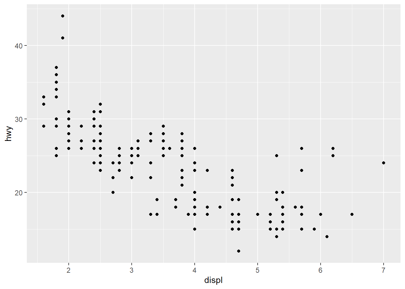
Before we use the above plot to propose an answer to our question, we should make a few comments about the code used to generate it.
ggplotis a function included in the tidyverse package for generating graphics in R.data =is the main argument toggplot, and it’s where you specify the data set your visualization is based on.- The
+sign at the end of the first row indicates that we’re adding a layer to our plot as defined by the next line. - The types of visualizations in tidyverse are known as geoms.
geom_pointis the scatter plot geom. We’ll see other geoms soon. mapping =is the main argument to a geom. It specifies how variables within the data set are mapped to various aesthetic features of the visualization.aesstands for aesthetic, and its arguments are the assignments of variables from the data set to various features (i.e., aesthetics) of the plot. In the above example,displis mapped to thexaesthetic (which defines what the x-axis represents) andhwyis mapped to theyaesthetic (which defines what the y-axis represents).
The scatter plot seems to indicate that, generally, the bigger a car’s engine is, the worse its fuel efficiency is.
Going forward, it will be necessary to distinguish between two types of variables. Consider the cyl variable, for example. Its values can be sorted into distinct categories: 4, 5, 6, and 8. We thus say that cyl is a categorical variable.
On the other hand, consider hwy. The values of this variable in mpg range from 12 to 44 and can potentially take on any value in that range. For example, it would make sense for hwy to take on a value such as 24.3 or any other number, integer or not, between some minimum and maximum. We thus say that hwy is a continuous variable.
Some categorical variables have values that can be ordered in some natural way. These are called ordinal categorical variables. The variable year in mpg is ordinal, for example. Other categorical variables have no natural way to order their values. These are called nominal categorical variables. The variable drv in mpg is nominal, for example.
Exercises
What would you expect a scatter plot showing the relationship between
hwyandctyto look like? Create such a plot.Classify each of the 11 variables in the
mpgdata set as either continuous or categorical. For each categorical variable, also determine whether it’s ordinal or nominal.Create a scatter plot to illustrate the relationship between fuel efficiency and a car’s drive train. What does your plot say about this relationship?
How is the plot from the previous problem qualitatively different from the plot of
hwyvs.displ? What accounts for this difference? (Hint: Think about what type of variabledrvis.)Scatter plots aren’t always appropriate ways to visualize relationships among variables. Get a scatter plot of
classvs.drvand explain why it’s not very useful. (Whenever we make statements like<VARIABLE>vs.<VARIABLE>, the first variable is considered to be the dependent (\(y\)-axis) variable and the second is the independent (\(x\)-axis) variable.)Explain why scatter plots are only appropriate when the
xandyaesthetics are both continuous variables.
1.2 Adding New Aesthetics to a Scatter Plot
There are some exceptions to the hwy vs. displ trend observed in the last section. Look at the points in the plot toward the upper right, which are cars with big engines and which yet have surprisingly high fuel efficiencies. Why might this be? What’s going on with these cars?
One conjecture might be that these are powerful cars (a consequence of a big engine) that are lightweight and aerodynamic (which implies better fuel efficiency). In other words, maybe they’re sports cars. Notice that the mpg data set contains a class variable. The sports cars are probably the ones for which the value of class is 2seater. One way to test this is by color-coding the points according to the class value. This is accomplished by assigning class to the color aesthetic:
ggplot(data = mpg) +
  geom_point(mapping = aes(x = displ, y = hwy, color = class))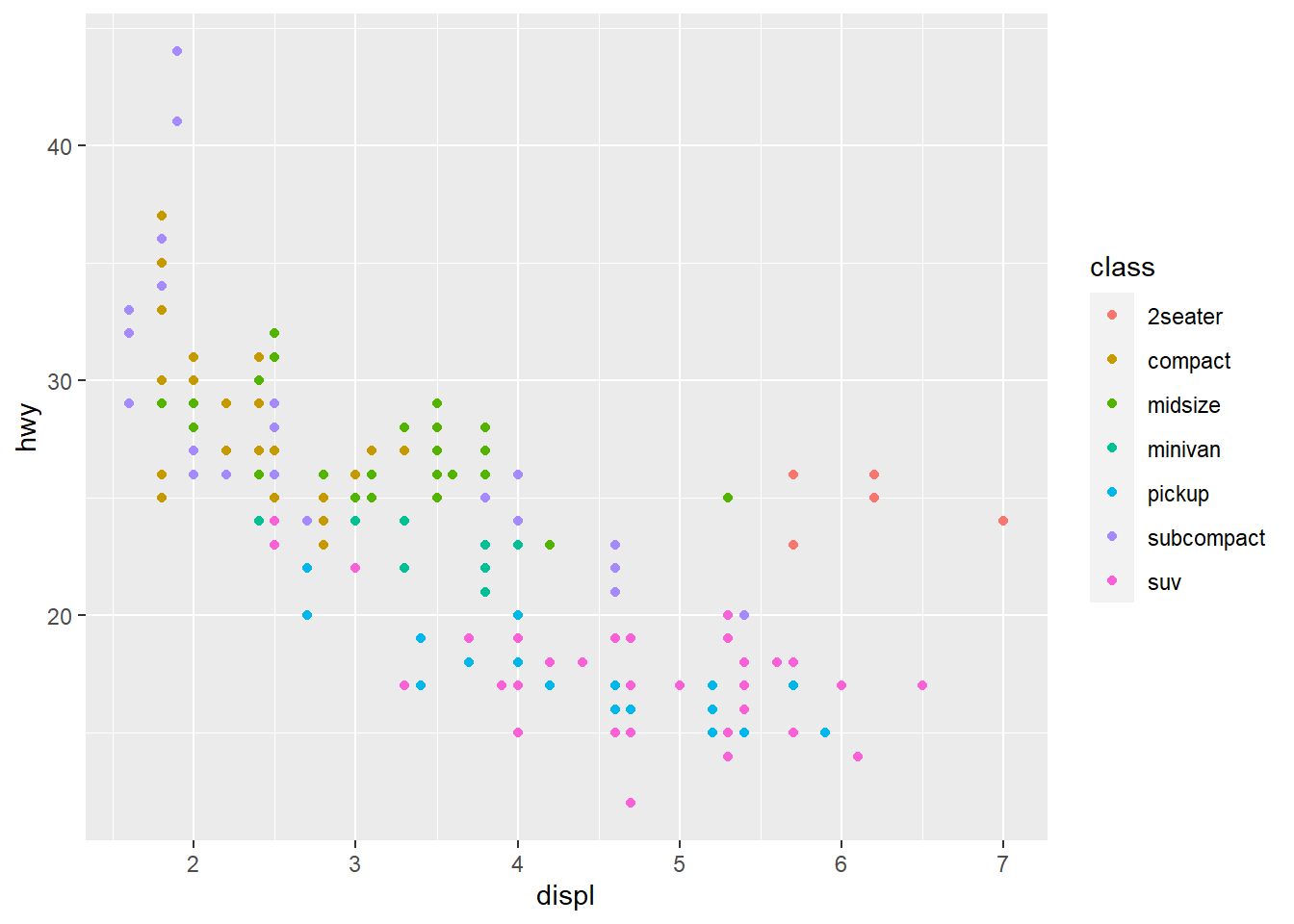
It seems we’re right; the pinkish-orange dots in the upper right indicate that these cars are sports cars. We also see that, as expected, SUvs. and pickup trucks don’t get good gas mileage even when their engines are relatively small and that the two cars with highway mileages above 40 miles per gallon are both subcompact cars (and likely even hybrids).
Each geom is equipped with several aesthetics. So far we’ve seen the x, y, and color aesthetics for geom_point. You can investigate others by reading the geom_point documentation:
?geom_pointThe exercises below will give you a chance to experiment with some of these aesthetics. As you’ll see, some aesthetics are designed for categorical and some for continuous variables.
Exercises
Obtain a scatter plot of
hwyvs.displ, but map the variableclassto the aestheticshaperather than tocolor. Why do you get a warning message?Re-do the previous problem, mapping a categorical variable with fewer categories than
classto theshapeaesthetic.What happens if you map a continuous variable to
shape?Try mapping variables, both continuous and categorical, to the
sizeaesthetic. What do you observe?What happens when you map a continuous variable to
color?Create a scatter plot with two extra aesthetics (in addition to
xandy). Don’t map the same variable to each one. Why might this not be considered a very good practice?Map a single variable to two different aesthetics. Why might this sometimes be a good idea?
Run the following code. Why might this be useful?
ggplot(data = mpg) +
  geom_point(mapping = aes(x = displ, y = hwy, color = cyl<6))
1.3 Labeling Visualizations
Recall our color-coded scatter plot from Section 1.2:

As it is, this plot would not be ready to include in a data analysis report because nothing is labeled. At a minimum, every visualization you create that someone else will see should have the following:
- meaningful labels for each axis
- meaningful labels for the legend (if applicable)
- the units of measurement for each variable used (if applicable)
These labels are inserted by adding another layer to the ggplot call. (Notice the + sign after the second line).
ggplot(mpg) +
  geom_point(mapping = aes(x = displ, y = hwy, color = class)) +
  labs(x = "engine displacement (L)",
       y = "highway fuel efficiency (mpg)",
       color = "type of vehicle")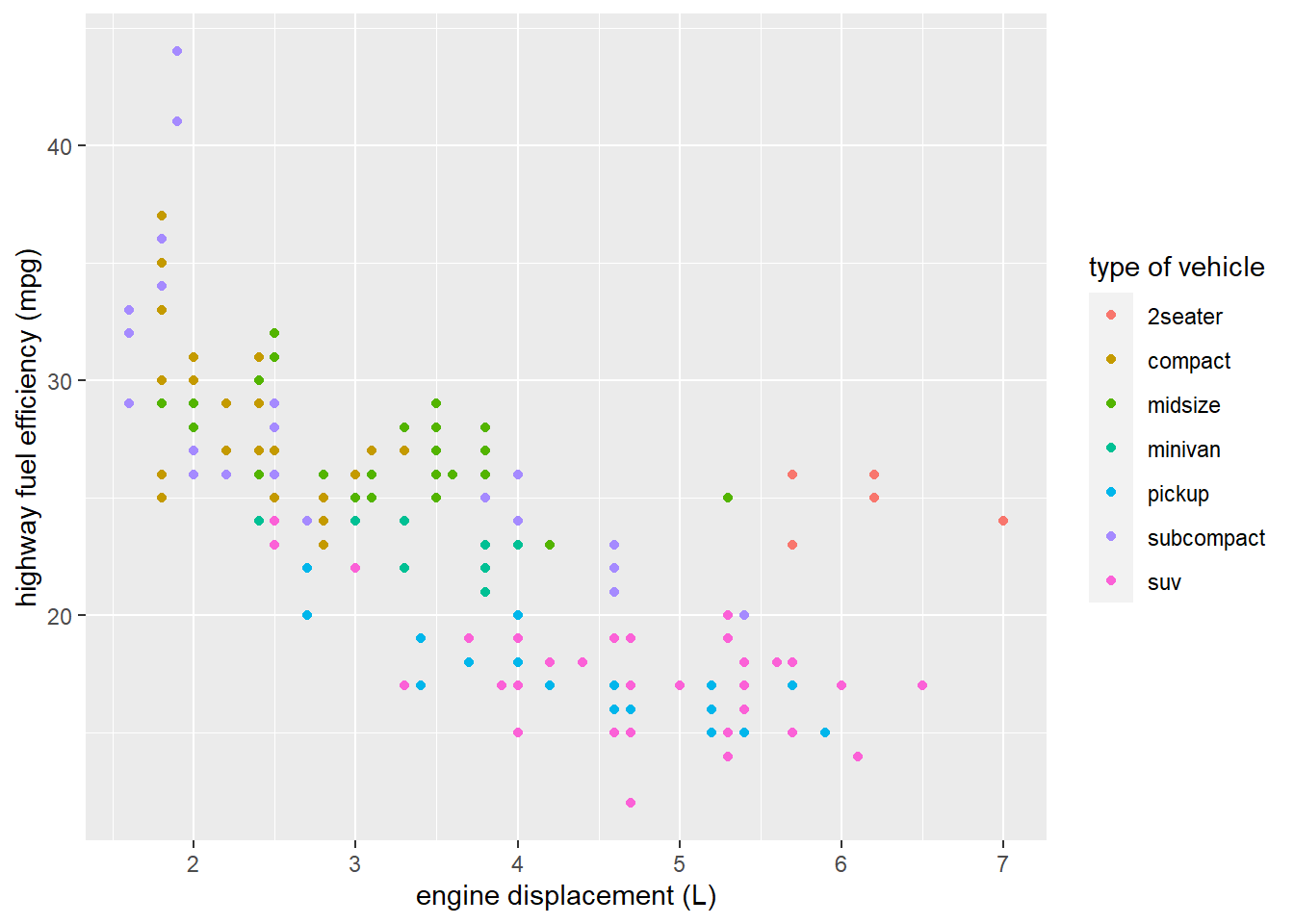
It’s often helpful to add other labels as well, including:
- a title (a general description of what your plot is supposed to display)
- a subtitle (a more detailed description; often omitted unless there’s a good reason to include one)
- a caption (a good place to say where your data comes from)
Here’s how to do it:
ggplot(mpg) +
  geom_point(mapping = aes(x = displ, y = hwy, color = class)) +
  labs(x = "engine displacement (L)",
       y = "highway fuel efficiency (mpg)",
       color = "type of vehicle",
       title = "Fuel Economy as a Function of Engine Size",
       subtitle = "Fuel Efficiency and Engine Size are Inversely Related",
       caption = "Data obtained from fueleconomy.gov")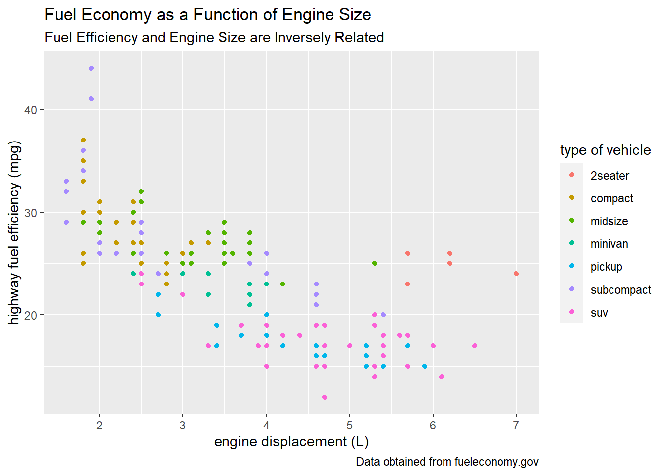
1.4 Trend Curves
Scatter plots are a good way to visualize a relationship between two continuous variables. Another way is to use a trend curve, which is accomplished with geom_smooth. We won’t worry about labels with any of the following examples, but remember that labels should always be included on visualizations when they’ll be viewed by others.
ggplot(data = mpg) +
  geom_smooth(mapping = aes(x = displ, y = hwy))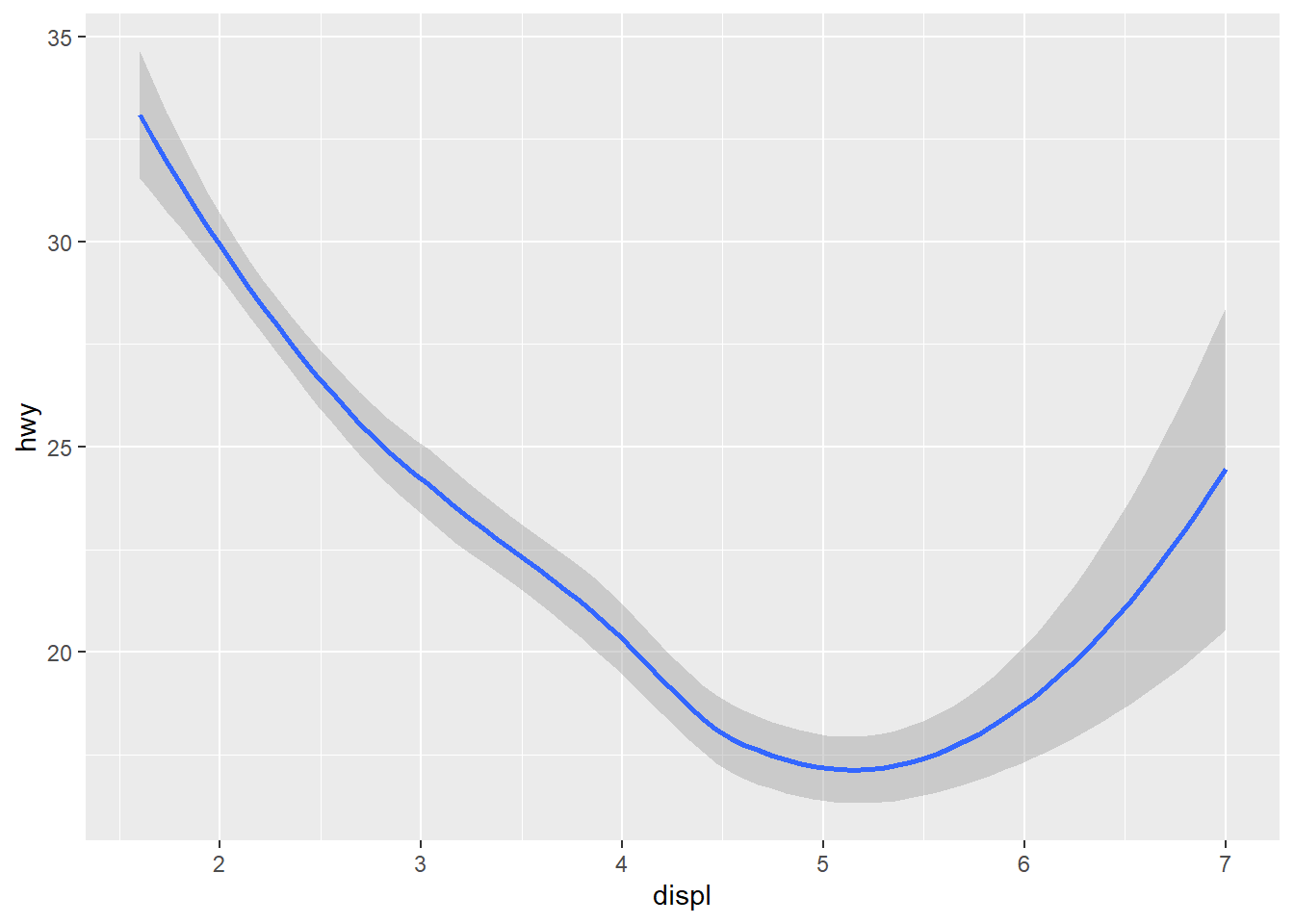
ggplot allows you to overlay multiple visualizations on the same graph. For example, trend curves are usually used in conjunction with scatter plots:
ggplot(data = mpg) +
  geom_point(mapping = aes(x = displ, y = hwy)) +
  geom_smooth(mapping = aes(x = displ, y = hwy))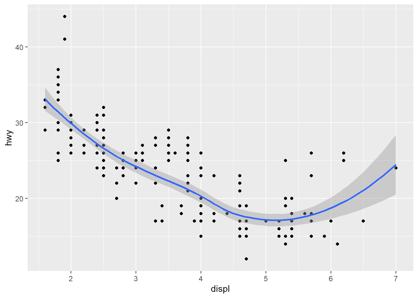
Notice that the code we used to generate the combined scatter plot and trend curve visualization has a lot of repetition. When all the layers in a visualization have a mapping in common, that mapping can be placed in the ggplot argument instead. For example, the following code produces the same plot as above:
ggplot(data = mpg, mapping = aes(x = displ, y = hwy)) +
  geom_point() +
  geom_smooth()
The gray band surrounding the curve represents a confidence interval, or more specifically, a 95% confidence interval. If we think of our data set as a sample of a larger population, then the trend curve we obtain is only an estimation of the true trend curve for the entire population. The gray band surrounding our trend curve represents the space in which we can be 95% certain that the true trend curve lies. The width of the confidence interval at a point on the curve is related to both the number and spread of the points in the scatter plot near that point. The narrow segments of the band correspond to parts of the scatter plot with many tightly clustered points (where we can be confident in our estimation), and the wide segments correspond to parts with only a few spread out points (where we can be less confident). The confidence interval can be turned off if desired by setting the se (which stands for “standard error”) argument to FALSE:
ggplot(data = mpg) +
  geom_smooth(mapping = aes(x = displ, y = hwy), se = FALSE)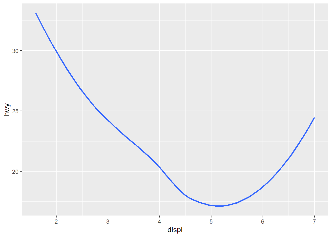
geom_smooth comes equipped with several aesthetics, which you can view in the documentation:
?geom_smoothYou can map variables to these aesthetics just like you did with geom_point. Here’s the color aesthetic:
ggplot(data = mpg) +
  geom_smooth(mapping = aes(x = displ, y = hwy, color = drv))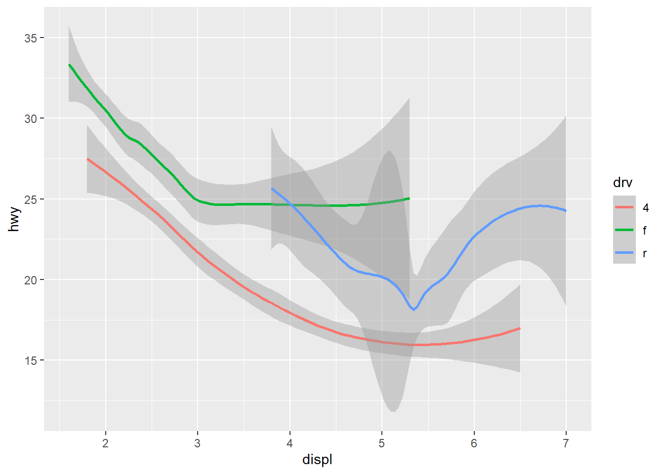
Apparently, it groups the data into the various categories of the drv variable and gives a separate curve for each category. This is a good way to compare trends among the different categories. (As you can see, color is an aesthetic suitable only for categorical variables.)
Sometimes we might want to specify that our trend curve be a straight line. This can be done by adding the method = lm argument to geom_smooth:
ggplot(data = mpg, mapping = aes(x = displ, y = hwy)) +
  geom_point() +
  geom_smooth(method = lm)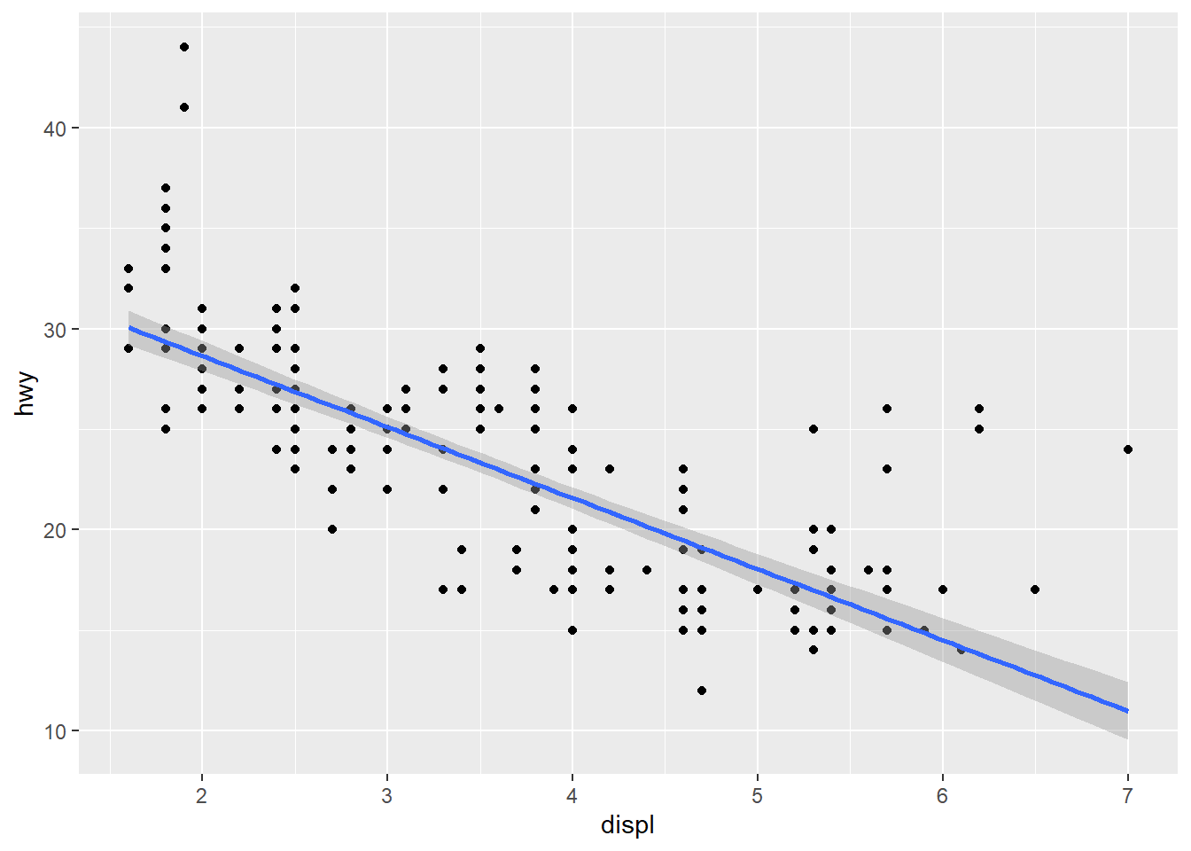
This line of best fit is called a regression line. We will examine linear regression in some depth in Chapter 4.
Exercises
Check the
geom_smoothdocumentation (?geom_smooth) to see some of the other aesthetics available besidescolor. Produce two different trend curve plots, each of which uses a different aesthetic. Display your plots and describe what your chosen aesthetics do.Obtain a single scatter plot that:
- shows the relationship between city fuel efficiency and highway fuel efficiency,
- color-codes the points by the type of drive train,
- has an overlaid regression line with no confidence interval, and
- has a title, properly labeled axes (including units), and a properly labeled legend.
Create a trend curve of
hwyvs.displand map theclassvariable tocolor. What do you think of your visualization? What recommendation would you make regarding mapping categorical variables tocolor?
1.5 Time Series Visualizations
A very common task of data analysts is to show how certain variables change over time. When a data set contains any kind of time variable (such as year, hour, quarter, month, etc.), we refer to it as time series data. A good way to visualize time series data is with a line graph.
The following data set gives home run totals in Major League Baseball by league every year from 1973 to 1995. Let’s analyze these home run totals as a time series. (This is not a built-in data set; running the following code chunk will import it from an external web site. We’ll learn how to import external data sets in Chapter 3.)
homeruns <- readr::read_csv("https://raw.githubusercontent.com/jafox11/MS282/main/homeruns.csv")homeruns## # A tibble: 46 x 3
## year league home_run_total
## <dbl> <chr> <dbl>
## 1 1973 AL 1552
## 2 1973 NL 1550
## 3 1974 AL 1369
## 4 1974 NL 1280
## 5 1975 AL 1465
## 6 1975 NL 1233
## 7 1976 AL 1122
## 8 1976 NL 1113
## 9 1977 AL 2013
## 10 1977 NL 1631
## # i 36 more rowsThe set up is the same as usual; the geom that produces a line graph is geom_line:
ggplot(data = homeruns) +
  geom_line(mapping = aes(x = year, y = home_run_total))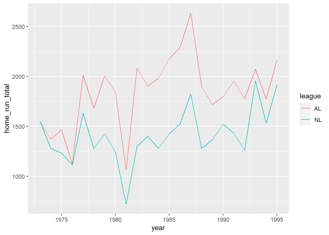
This doesn’t look right. If you look carefully, you’ll notice that there’s a vertical line segment above each year. This is because each year in the data set is entered twice, once for each league. It would be better to get separate line graphs for each league so that we can compare. This is easily accomplished by mapping the league variable to the color aesthetic:
ggplot(data = homeruns) +
  geom_line(mapping = aes(x = year, y = home_run_total, color = league))
It’s often helpful to overlay a scatter plot on top of the line graph. Notice that we can move the mapping argument up to the ggplot line since it applies to both geoms.
ggplot(data = homeruns, mapping = aes(x = year, y = home_run_total, color = league)) +
  geom_line() +
  geom_point()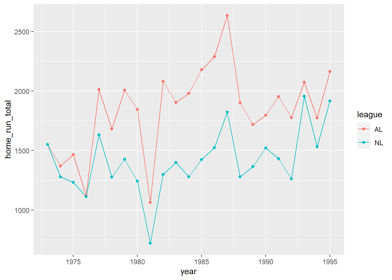
Line graphs are nice for time series analyses because the lines that join successive points make it easier to visually follow changes over time. For example, there are features in the line graph above that raise very natural questions and give us an opportunity to “tell a story” about the data.
- Q: Why is it that from 1973 onward, the American League always hit more home runs than the National League?
A: It turns out that in 1973, the American League instituted the designated hitter rule. This allowed teams to substitute a player to hit in place of the pitcher. Given that pitchers rarely hit home runs, using a designated hitter in the AL probably caused home run totals to increase. - Q: Why did the gap between the American and National Leagues widen so much in 1977 and then shrink again in 1993?
A: In 1977, the American League added two new teams (the Seattle Mariners and Toronto Blue Jays). This gave the AL 14 teams, while the NL only had 12. Thus, it makes sense that more home runs would be hit in the AL. In 1993, the NL expanded to 14 teams (adding the Colorado Rockies and Florida Marlins), so the gap closed again. - Q: Why was there such a big dip in home runs in 1981?
A: There was a players strike in 1981, and about 40% of all games were canceled.
Exercises
Run the following line of code to load the data set needed for these exercises:
SuperBowl <- readr::read_csv("https://raw.githubusercontent.com/jafox11/MS282/main/SuperBowl.csv")This contains data related to Super Bowl viewership and advertisement costs every year since 1967. The Viewers variable is the number of people who watched the Super Bowl on TV (in millions), AdCost is the average cost of running a 30-second advertisement during the game, and AdCost2023 is the average advertisement cost adjusted for inflation (expressed in 2023 dollars).
Create a line graph (together with a scatter plot) that shows how Super Bowl viewership changed over time. Then speculate on any unusual features of the line graph (such as sharp decreases or increases).
Create a line graph (together with a scatter plot) that shows how the average advertisement cost changed over time.
Modify your visualization from the previous exercise so that the points in the scatter plot are color-coded in a way that indicates whether there were over 100 million viewers. (See Exercise 8 in Section 1.2.)
Based on your visualization from the previous exercise, indicate a few years when advertisers were probably disappointed by the number of viewers.
1.6 Box Plots
In Exercise 4 in Section 1.1, we considered the following scatter plot:
ggplot(data = mpg) +
  geom_point(mapping = aes(x = drv, y = hwy))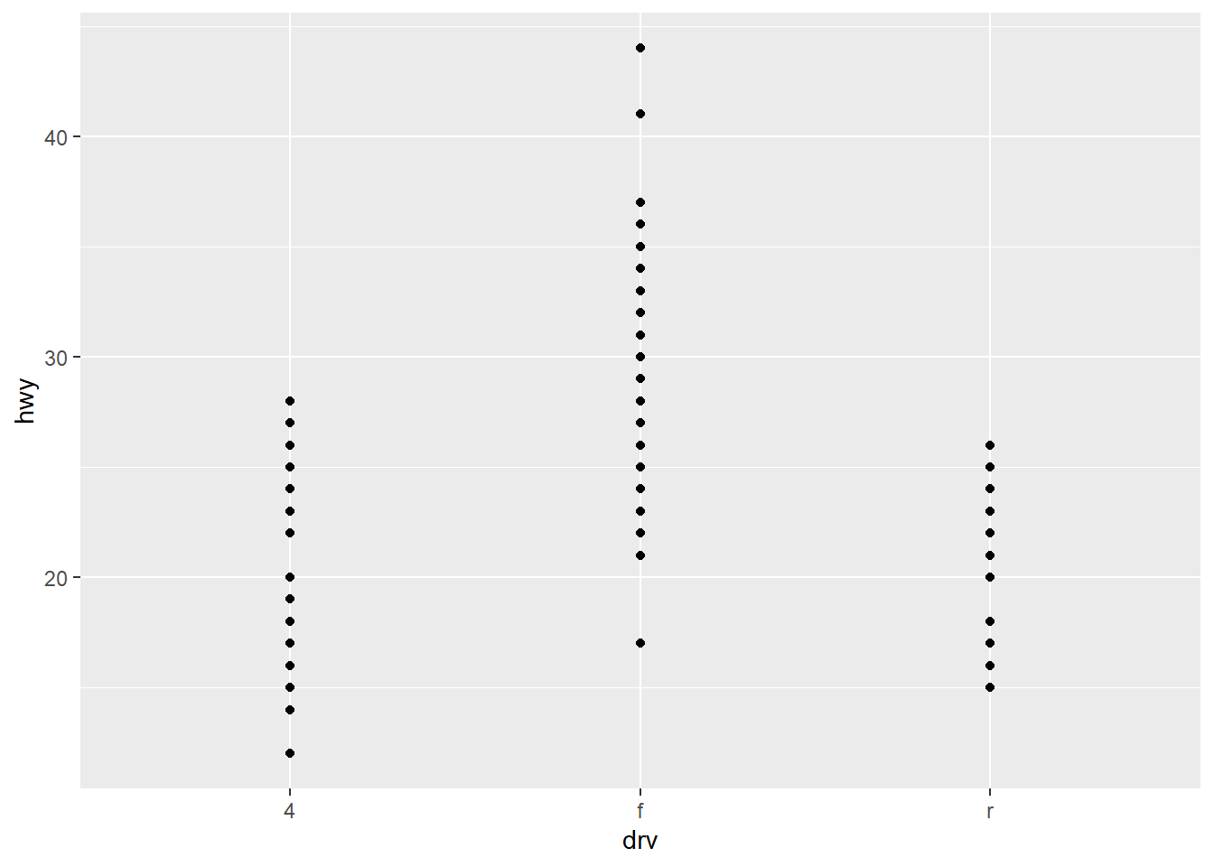
The point of that exercise was to show that scatter plots are not the right visualization to use when either of the variables is categorical. A much better option is a box plot. Before we see how these are created, there are a few terms to define.
The median of a continuous variable is the number in the middle position (when put in numerical order) if there are an odd number of points or the average of the two middle numbers if there are an even number of points. For example, in an ordered data set with 11 points, the median is the 6th point in the list. If there are 24 points, the median is the average of the 12th and 13th points. The median of a data set has the property that 50% of the points are less than or equal to the median and 50% are greater than or equal to it.
Given a continuous variable, the first quartile (Q1) is, like the median, a cut point in the variable’s values. It divides the data points into the smallest 25% and the largest 75%. The third quartile (Q3) is a cut point which divides the list into the smallest 75% and the largest 25%. (The second quartile (Q2) is just the median.) The data that lies between Q1 and Q3 thus comprises about 50% of the data in the set.
The interquartile range (IQR) is the value of Q3 \(-\) Q1.
Example: Suppose our data set consists of the points 32.1, 56.3, 27.2, 6.7, 56.5, 24.7, 12.9, 35.8, 54.1, and 71.1. To find the median and quartiles, we first have to put the numbers in order: 6.7, 12.9, 24.7, 27.2, 32.1, 35.8, 54.1, 56.3, 56.5, 71.1. Since there are 10 data points, the median is the average of the 5th and 6th numbers: 33.95.
Since our 10 data points cannot be divided into groups of 4, we cannot find Q1 and Q3 exactly. There are actually several competing methods for finding quartiles in this case. To avoid too much of a detour, we will use R to compute quartiles. As you can see below, the way to enter a list of data points in R is to enter them into a character vector: c(<VALUE>, <VALUE>, . . .).
x <- c(32.1, 56.3, 27.2, 6.7, 56.5, 24.7, 12.9, 35.8, 54.1, 71.1)
quantile(x, probs = c(0.25, 0.50, 0.75))
## 25% 50% 75%
## 25.325 33.950 55.750We thus see that Q1 = 25.325, Q2 = 33.95 (which we already knew), and Q3 = 55.75. The IQR is 55.75 \(-\) 25.325 = 30.425.
The code above refers to the fact that quartiles are actually specific examples of quantiles. Quantiles are a set of cut points that divide a numerical data set into specified percentiles. Quartiles are therefore quantiles for which the percentiles are 25%, 50%, and 75%.
We are now finally ready to create and interpret a box plot. The set-up is similar to that of scatter plots, trend curves, and line graphs; the new geom to use is geom_boxplot:
ggplot(data = mpg) +
  geom_boxplot(mapping = aes(x = drv, y = hwy))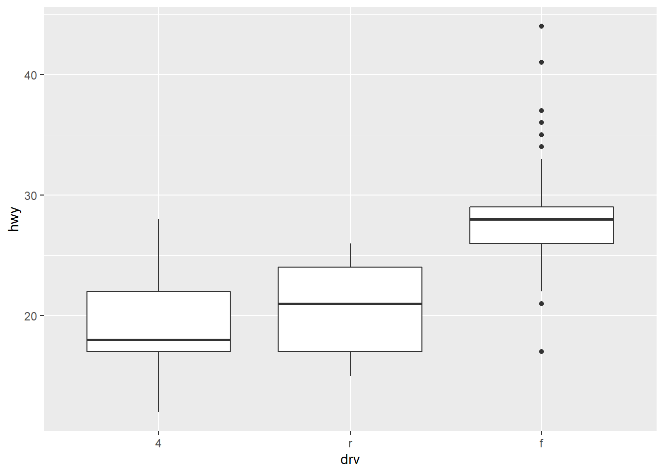
For each of the possible values of drv (4, f, and r), we get a diagram interpreted as follows:
The horizontal line inside the box is drawn at the median value of
hwyfor the given value ofdrv.The top horizontal line is drawn at the third quartile, and the bottom horizontal line is drawn at the first quartile.
The dots above and below the vertical lines represent outliers, which are data points that are extremely large or small relative to the rest of the data. There are several ways to determine which data points are to be considered outliers. The method used here is to consider outliers to be data points that are greater than Q3 \(+\) 1.5 \(\times\) IQR or less than Q1 \(-\) 1.5 \(\times\) IQR.
The vertical line above the box extends to the largest non-outlier, and the one below extends to the smallest non-outlier.
The above plot of hwy vs. drv thus shows that:
Cars with front-wheel drive tend to get the best highway gas mileage but also that there’s a lot of variation among the values of
hwyin that group, especially beyond the interquartile range.Cars with rear-wheel drive have a larger interquartile range, but the values of
hwydon’t stray very far outside that range.Cars with 4-wheel drive have a median value that is much closer to Q1 than to Q3, which suggests that the values of
hwyabove the median are significantly farther from the median than those below.
It’s often helpful to produce box plots in which the boxes are displayed in ascending or descending order of height. For the box plot above, this would mean switching the boxes for r and f. We can do this automatically by specifying that we want to reorder the boxes so that the drv variable is ordered according to its mean value of hwy. Here’s how to do this:
ggplot(data = mpg) +
  geom_boxplot(mapping = aes(x = reorder(drv,hwy), y = hwy)) +
  labs(x = "drv")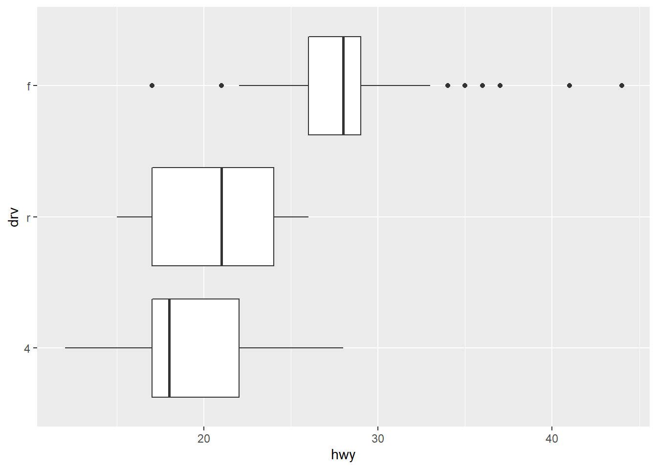
(In case you’re wondering why we added an x-axis label to the reordered box plot above, try running the ggplot call without the labs layer and see what happens.)
Another option we have with box plots is to flip them so that the boxes are displayed horizontally. This is especially helpful when the categorical variable has a lot of values crowded onto the x-axis. We can do this by adding a coord_flip() layer:
ggplot(data = mpg) +
  geom_boxplot(mapping = aes(x = reorder(drv, hwy), y = hwy)) +
  labs(x = "drv") +
  coord_flip()
Box plots also come equipped with various aesthetics, which you’ll explore in the exercises. The main thing to remember about box plots, though, is that they’re a good way to visualize how a continuous variable depends on a categorical one.
Exercises
These exercises will make use of the built-in diamonds data set. First take a few minutes to look through the data set and read the documentation.
View(diamonds)
?diamonds
Obtain a visualization that shows the relationship between
caratandprice. (Pay attention to the types of variables you’re using so that you create the appropriate type of visualization.)Repeat the previous exercise, but replace
caratwithclarity. (Be careful, you might not be able to use the same type of visualization as in the previous problem.)According to your plot from the previous exercise, which type of clarity is priced the highest? Which type has the most variation in price?
Referring again to the plot from Exercise 2, why do you think all of the outliers are above the main cluster of data points?
Obtain a box plot of
pricevs.color. Three of the aesthetics included ingeom_boxplotarecolor,fill, andlinetype. Using three different plots, try mapping thecutvariable to each of these aesthetics. Which of these three (in your opinion) is the most effective way to distinguish among different diamond cuts in your box plot and why?Re-do Exercise 2, but display the boxes horizontally, arranged by average
pricevalue. (Remember to adjust the axis label appropriately after reordering.)
1.7 Visualizing Distributions: Bar Graphs and Histograms
The visualizations we’ve seen so far – scatter plots, trend curves, line graphs, and box plots – are ways to display covariation among two variables. This means that they show how changes in one variable are related to changes in another variable. In this section, we look at ways to visualize how values of a single variable vary; in other words, we will see how to visualize a variable’s distribution. The two primary visualizations for distributions are bar graphs (for categorical variables) and histograms (for continuous variables).
Bar graphs and histograms both visualize how a single variable is distributed by providing a count of how many times each value of the variable is attained. We’ll start with bar graphs. Notice that we only have to provide an x mapping; the y variable in the plot is the value count:
ggplot(data = diamonds) +
  geom_bar(mapping = aes(x = cut))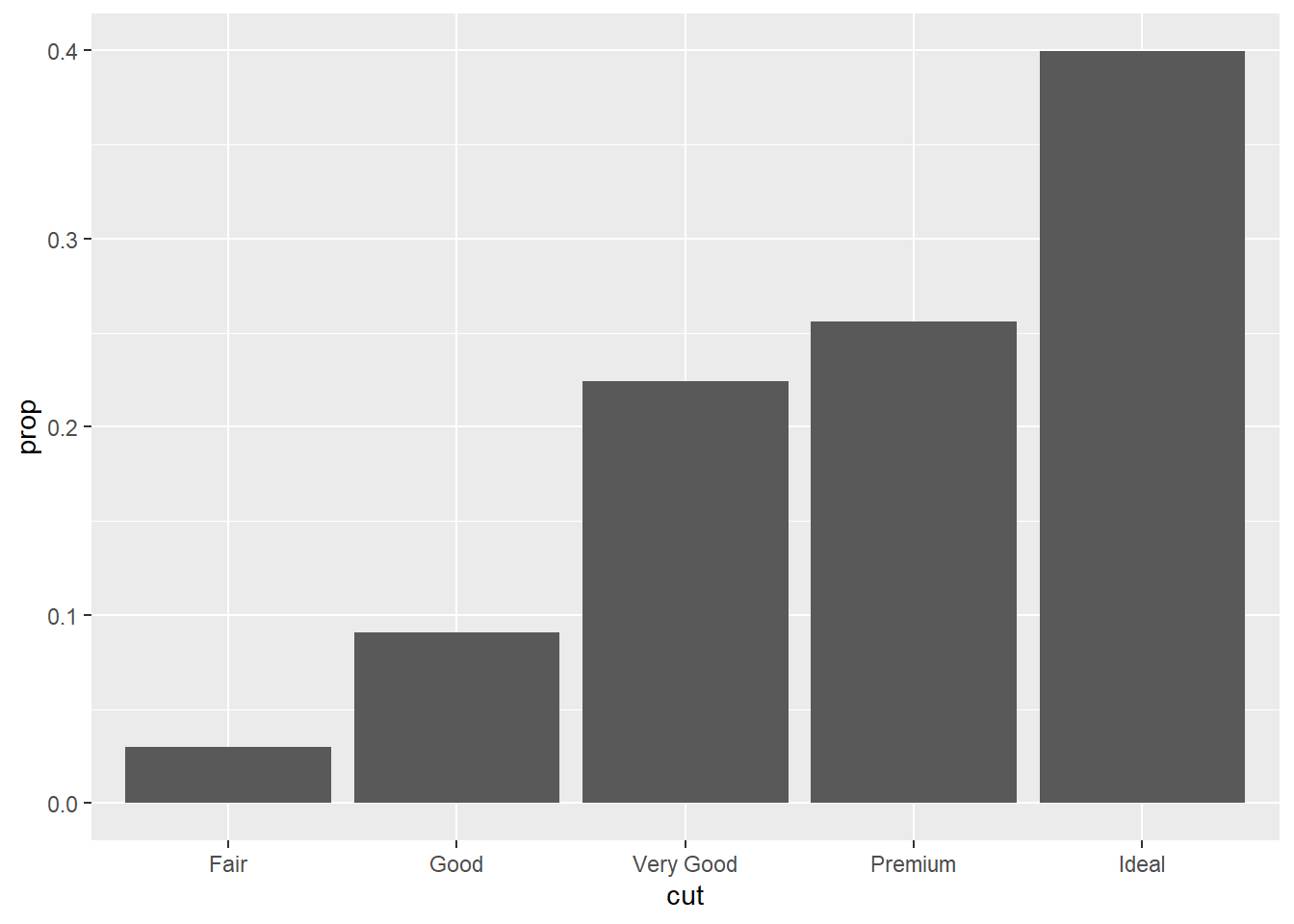
We see that diamonds with an ideal cut are the most numerous in the set. Sometimes it’s preferable to have a bar graph show the percentages that each category makes up in the data set. In this case, we can think of the bar graph as representing a probability distribution of the different categories. We can override the default mapping of count to y by instead mapping the proportion stat(prop):
ggplot(data = diamonds) +
  geom_bar(mapping = aes(x = cut, y = stat(prop), group = 1))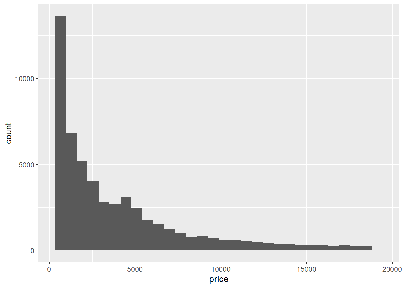
The group = 1 mapping is included to make sure that the proportions calculated by stat(prop) are relative to the entire data set, not just relative to each category. (Try running the code above without group = 1 and see what happens.)
Anyway, from the above bar graph, we can read off how likely it is to choose any category randomly. For example, it looks like we have about a 22% chance of selecting a “Very Good” diamond at random.
Histograms serve the same purpose as bar graphs but are used for continuous, rather than categorical, variables. The problem with continuous data is that we don’t want to count how many times each value of a variable shows up; there would be way too many such values and thus way too many bars in the bar graph.
We solve the problem of visualizing a continuous distribution by binning. Binning is the process of subdividing the continuous interval of values, stretching from the minimum value to the maximum, into subintervals (or bins). Each bin is then treated like a category, and a count of the number of values in each bin is made and used to determine the height of a bar (just like in a bar graph). The default in ggplot is to use 30 bins.
ggplot(data = diamonds) +
  geom_histogram(mapping = aes(x = price))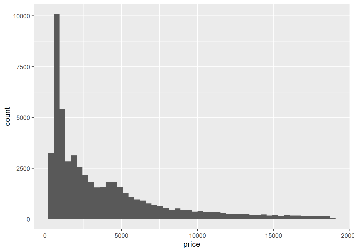
You can override the default number of bins by either specifying how many bins you want or by specifying how wide you want your bins to be:
ggplot(data = diamonds) +
  geom_histogram(mapping = aes(x = price), bins = 50)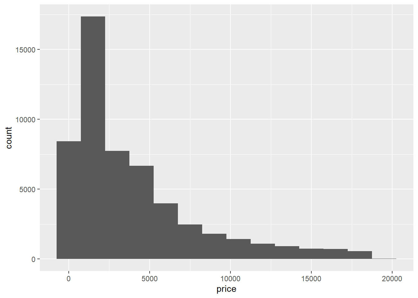
ggplot(data = diamonds) +
  geom_histogram(mapping = aes(x = price), binwidth = 1500)
Choosing the number of bins in a histogram is a subtle art; you don’t want them to be so wide that they make the distribution look too coarse, and you don’t want them to be so narrow that they make the distribution look too fine or “granular.”
Both geom_bar and geom_histogram have several aesthetics, which you’ll explore in the exercises.
Exercises
Create a visualization of the distribution of the
clarityvariable indiamonds. (Be sure to use the appropriate geom for this type of variable.)Re-do the previous problem, but have the y-axis record the percentages of each
clarityvalue withindiamonds.Create a visualization of the distribution of the
caratvariable indiamonds. (Be sure to use the appropriate geom for this type of variable.)
- Create a histogram for which the bins are way too narrow. Then create one for which they’re way too wide. What do you observe in each case?
Two useful aesthetics for bar graphs are
colorandfill. For your bar graph from Exercise 1 above, try mappingcuttocolorand then tofill. Which seems to be the more helpful aesthetic?A more useful way to apply the
colororfillaesthetics is to pair them with the optionalpositionargument. Run the following code and reflect on how the bar graph might be better than the ones from Exercise 5.
ggplot(data = diamonds) +
geom_bar(mapping = aes(x = clarity, fill = cut), position = "dodge")- Explain why the following code would produce a bar graph that would contain some redundancy but would also be visually pleasing:
ggplot(data = diamonds) +
  geom_bar(mapping = aes(x = cut, fill = cut))
Reproduce the bar graph from the previous problem, but add an extra layer:
+ coord_polar(). What happens?Create a visualization of the distribution of the
manufacturervariable inmpg. Explain why this visualization would look better if the bars were displayed horizontally rather than vertically, then create such a visualization. (Hint: Recall how this is done for box plots.)The aesthetics for
geom_histogramare the same as those forgeom_bar. Create a histogram that shows the distribution ofcaratwithindiamondsand use an aesthetic to show the distribution ofcutvalues within each bin.A geom very similar to
geom_histogramisgeom_freqpoly(which stands for frequency polygon). Create a visualization of the distribution ofpricewithindiamondsusinggeom_freqpolyinstead ofgeom_histogram. Why might this sometimes be preferable to a histogram?As you may have seen in Exercise 10, you can map an extra variable to the
colororfillaesthetic, but the result is somewhat visually confusing. Retry Exercise 10, but usegeom_freqpolyrather thangeom_histogram. Do you think this is a better visualization?Using the
mpgdata set, create a visualization of the distribution of types of cars in the data set, and include a breakdown of the distribution of drive trains present for each type of car. Label the x- and y-axes and the legend with meaningful names, and give your plot an appropriate title.
1.8 Summary
There are thousands of combinations of visualizations and aesthetics available for ggplot, and these visualizations are almost infinitely customizable. We’ve only scratched the very outermost surface here by seeing how a few commonly used visualizations are produced.
However, for each visualization, the basic grammar is the same:
ggplot(data = <DATASET>) +
  geom_<GEOM TYPE>(mapping = aes(<MAPPINGS>), position = <POSITION>) +
  <NEXT GEOM LAYER> +
  <NEXT GEOM LAYER> +
  <ETC> +
  <COORDINATES>
And the visualizations we’ve seen at this point are:
| geom | x |
y |
|---|---|---|
| scatter plot | continuous | continuous |
| trend curve | continuous | continuous |
| line graph | time variable | continuous |
| box plot | categorical | continuous |
| bar graph | categorical | count or proportion |
| histogram | continuous | count or proportion |
| frequency polygon | continuous | count or proportion |
1.9 More about R Notebooks
As we have seen, R Notebooks are a good way to mix code with written narrative, and this makes them ideal for preparing professional data analysis reports using R. Before preparing our first such report, it will be necessary to learn a few more features of R Notebooks and R Markdown formatting.
Code Chunk Settings
A code chunk in an R Notebook has the following basic structure:
```{r <OPTIONAL NAME OF CHUNK>, <OPTIONAL SETTINGS>}
<CODE GOES HERE>
```
Sometimes it might be necessary to hide the code and/or output of a code chunk for the purpose of producing a professional looking report. This can be done by adjusting the settings of the code chunk where it says <OPTIONAL SETTINGS> in the sample above. Here are some common settings:
include=FALSEprevents both the code and the code’s output from appearing in the compiled document.echo=FALSEprevents the code, but not the output, from appearing.eval=FALSEprevents the output, but not the code, from appearing.message=FALSEprevents any messages generated with the output from appearing.warning=FALSEprevents any warnings generated with the output from appearing.
For example, suppose we want to prevent a code chunk from showing up in the compiled document, but we still want its output to be displayed. However, suppose we don’t want any messages or warnings to appear with the output. We would adjust the code chunk’s settings as follows:
```{r <OPTIONAL NAME OF CHUNK>, echo=FALSE, message=FALSE, warning=FALSE}
<CODE GOES HERE>
```
Since you will almost never want messages or warnings to show up in your compiled document, you can set these options globally at the beginning of your .Rmd file. After the --- that follows your title, name, date, output, etc, just enter the following code chunk. Then you won’t have to turn off messages and warnings within each individual chunk.
```{r, include=FALSE}
knitr::opts_chunk$set(message=FALSE, warning=FALSE)
```
There are other settings that might come in handy as well. There is also a lot of formatting syntax used in R Markdown, including ways to create bold font, italics, bulleted lists, hyperlinks, etc. Your best bet is to Google “how to ______ in R Markdown” when you need to apply some kind of formatting.
Displaying Data Sets
It’s a good practice to show at least part of the data set you’re using in your analysis report. However, if you try our usual View(<DATA SET>) in an R Notebook file, nothing shows up. Instead, use the datatable function from the DT package. You’ll first have to install this package, although don’t do it in an R Markdown code chunk. Do it in any R script file.
install.packages("DT")Then load the DT library in your R Notebook file. You could do this right after you load tidyverse:
library(DT)The following code shows how to use the datatable function. The options = list(scrollX = TRUE) argument ensures that if the data table is too wide for the screen, a horizontal scroll bar will be provided in the compiled document. If you put this in a code chunk in an R Notebook file, the data table will appear in your report as it is seen below.
datatable(mpg, options = list(scrollX = TRUE))Publishing Reports on the Internet
Once your R Notebook has been compiled into an HTML file, it’s easy to upload it to the internet (for free) using the web site RPubs, which is part of RStudio. Your file is assigned its own URL, which you can then easily share with anyone or even include on a resume. Here are the steps for publishing your reports online:
- Knit your Rmd file to an HTML file.
- When your HTML file pops up, click the “Publish” button in the upper right corner of the window.
- On the screen that opens, choose “RPubs.”
- On the next screen, click “Publish.”
- On the next screen, either create an RPubs account or log in to your existing account. When you create an account, be aware that your username will be a part of your URL, so choose a professional-sounding username.
- On the next screen, you can choose a title for your document and enter a description. These show up on your project dashboard, so other people will see these. You can also choose a “slug” for your URL, which is a word or phrase that will also show up in your URL. Click “Continue” when you’re done.
- You now have a published R report online! You can share the URL with anyone. If you ever need to update your publsihed report, you can unpublish it and upload an updated version.
1.10 Project
Project Description: The purpose of this project is to use ggplot and its various geoms to answer questions about a data set by creating meaningful and aesthetically pleasing visualizations.
In particular, we will be analyzing data relating to the tv show The Office, which, as everyone knows, is the best show of all time. You can import the data set by executing all three commands in the following code chunk. (The data set is a compilation of the ones found here and here.)
office_ratings <- readr::read_csv('https://raw.githubusercontent.com/jafox11/MS282/main/office_ratings.csv')
office_ratings$season <- as.character(office_ratings$season)
office_ratings$air_date <- as.Date(office_ratings$air_date, "%m/%d/%Y")
The name of the data set to which you’ll refer is office_ratings. And here’s the data dictionary:
| variable | variable type | description |
|---|---|---|
season |
categorical | season during which the episode aired |
episode |
categorical | episode number within the season |
title |
categorical | title of episode |
viewers |
continuous | number of viewers in millions on original air date |
imdb_rating |
continuous | average fan rating on IMDb.com from 1 to 10 |
total_votes |
continuous | number of ratings on IMDb.com |
air_date |
date | date episode originally aired |
Instructions:
Use well-chosen visualizations to answer the following questions.
How are each of the three continuous variables distributed? (Where is the peak and what does it tell you? What does the shape of the distribution tell you? Are there any extreme values?)
Is it the case that the more people watch an episode, the better it’s liked?
Are there any exceptions to the trend you noticed in the previous problem? Use a visualization to try to explain these exceptions.
Is it the case that the more people watch an episode, the more people leave an IMDb rating? Are there exceptions? If so, use a visualization to try to explain them.
How did the show’s popularity change over time?
How did the show’s appeal change over time? (Be careful, popularity and appeal are not the same thing. Think about which variables address these two attributes.)
In the previous two problems, you should notice that the show’s popularity and appeal don’t change in exactly the same way throughout the series. Use the differences you notice in the visualizations to explain why this might be.
Is there a trend in total viewership within the individual seasons? Are there any notable changes in viewership within any season? If so, can you explain the reason for these changes?
Guidelines:
Heading: Include a descriptive title for your report (do not just call it “Project 1”), your name, and the date in the heading.
Introduction:
- Begin with a description of the problem you’re solving or question you’re answering in your report. This should be concise but detailed enough to set the stage for the work you’ll be doing.
- Describe your data set. Say what it contains, how many observations and variables it contains, and where it comes from.
- Create a data dictionary, at least for the variables which will be referenced in your report.
- Use the
datatablefunction to display your data set. (If the data set is too big to display when you try to knit your .Rmd file, you don’t have to display it.) - Include a code chunk in which you load the libraries you’ll need, and briefly say what each one is for.
Body:
- Follow the introduction with the body of your report which will contain your work, broken into relevant section headings.
- The body should include text that provides a running narrative that guides the reader through your work. This should be thorough and complete, but you should avoid large blocks of text.
- Do not use the problem-numbering in the Instructions above in the body. That’s just for your benefit as you prepare your work. Your narrative structure – not an enumerated list – should lead the reader from one question to the next.
- The body of the report should show all of your R code and its output, but it should not show any warning or error messages. (This is for my benefit. A professional report might not include the code, depending on the audience.)
- All graphics should look nice, be easy to read, and be fully labeled.
- You should include insightful statements about the meaning you’re extracting from your graphics rather than just superficial descriptions of your visualizations.
Conclusion:
- End with an overall concluding statement which summarizes your findings.
- Provide a clear answer to the question you set out to answer.
- If you were not able to answer the question fully, possibly because of insufficient data, explain why.
Report Preparation: The problems for the project should be worked out in a scratch work .R file which you will not turn in. Once you’re done, write up your results in an R Notebook report, making sure to follow the guidelines above. Then publish your report online using RPubs and send me the URL to submit your work.
Grading Rubric:
Graphics: Do the graphics convey meaning? Do they look nice? Are they fully labeled? Are the geoms used appropriate for the data being displayed? (30 points)
Insights: Are insights fully explained, well-written, and significant (i.e., not superficial)? Are your insights derived from the graphics? (30 points)
Narrative: Is it clear what you’re trying to do in this project? Do you maintain a readable narrative throughout that guides the reader through your analysis? (20 points)
Professionalism: Does your report look nice? Do you provide insights based on your analysis? Is your code clear and readable? Did you follow the guidelines listed above? (15 points)
You can see a short sample report here. You can also download the source .Rmd file here to use as a template.